If you have read three articles about "AI" this week, you have probably seen the words AI, machine learning, deep learning and generative AI used as if they meant the same thing. They do not, and mixing them up is the fastest way to sound confused in an interview. The good news is that the relationship is simple. It is four circles, each inside the one before.
After we sort the vocabulary out, we build the first real model of the course, linear regression. It is the oldest, simplest and most useful starting point in machine learning, and nearly every later idea in this roadmap is a reaction to something it cannot do. You should already be comfortable with the train/test split from Session 1. If you are not, spend ten minutes there first.
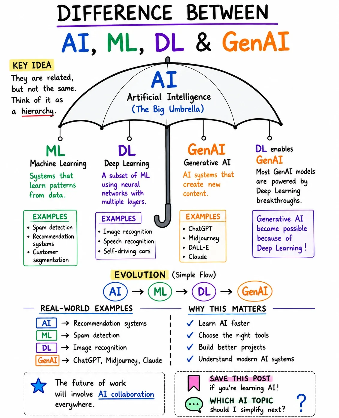
The four terms, one inside the other

Artificial intelligence (AI) is the widest idea: getting machines to do things that normally need human intelligence. It does not say how. A chess program that checks thousands of positions using rules a programmer typed in counts as AI, even though it never learns anything.
Machine learning (ML) is one way of building AI. Instead of writing the rules, you show the computer many examples and let it find the pattern itself. A spam filter is the classic case. Nobody lists every spammy phrase. The model looks at thousands of labelled emails and learns which words, senders and links go with junk. In classic ML, a person still decides which clues to feed it, for example "number of links" or "sender seen before".
Deep learning (DL) is a kind of ML that uses neural networks with many layers. Its strength is that it learns the clues too. Show a face-unlock model raw pixels and it works out edges, then shapes, then eyes and noses, without anyone defining what an eye is. This is why deep learning took over images, speech and text.
Generative AI (GenAI) is deep learning that creates. Instead of putting an email in a "spam" or "not spam" box, it writes the next sentence, draws a picture or composes a tune. ChatGPT, Claude and image generators are all in this circle.
| What it is | Who picks the features? | Real example | |
|---|---|---|---|
| AI | Machines doing tasks that need intelligence | Not specified | A rule-based chess engine |
| ML | Learning patterns from data | A human | A spam filter |
| DL | ML with deep neural networks | The network, from raw data | Phone face unlock |
| GenAI | DL that produces new content | The network | A chatbot, an image generator |
The phrase "artificial intelligence" comes from a 1955 proposal for a summer workshop at Dartmouth College, held in 1956. It was written by John McCarthy, Marvin Minsky, Nathaniel Rochester and Claude Shannon.Dartmouth AI proposal, 1955
ChatGPT launched on 30 November 2022. OpenAI itself had been founded seven years earlier, in December 2015.OpenAI announcements
Three ways a machine can learn
The word "learning" covers three setups, and the course touches all of them:
- Supervised learning. Every example comes with the right answer, and the model learns to reproduce it. House prices from features, spam or not spam. Most of this roadmap.
- Unsupervised learning. No answers, only data. The model looks for structure, like grouping customers into types (Session 9).
- Reinforcement learning. An agent tries actions, gets rewards or penalties and improves by trial and error. It is how game-playing systems learned, and a flavour of it is used when chat models are tuned to be helpful.
Regression or classification?
Before you pick a model, look at what you are predicting. If the answer is a number on a scale (a price, a temperature, a mark out of 100), the task is regression. If it is one of a few labels (spam or not, which digit, which disease), it is classification. Text-based categories have to be turned into numbers first, which you saw with one-hot encoding in Session 1.
Linear regression in one picture
Imagine a street stall that sells kulfi in Karachi. On hot days sales go up, on cool days they drop. Plot temperature against sales and the dots drift upward. Linear regression draws the single straight line that sits closest to all of them, and then uses that line to predict.
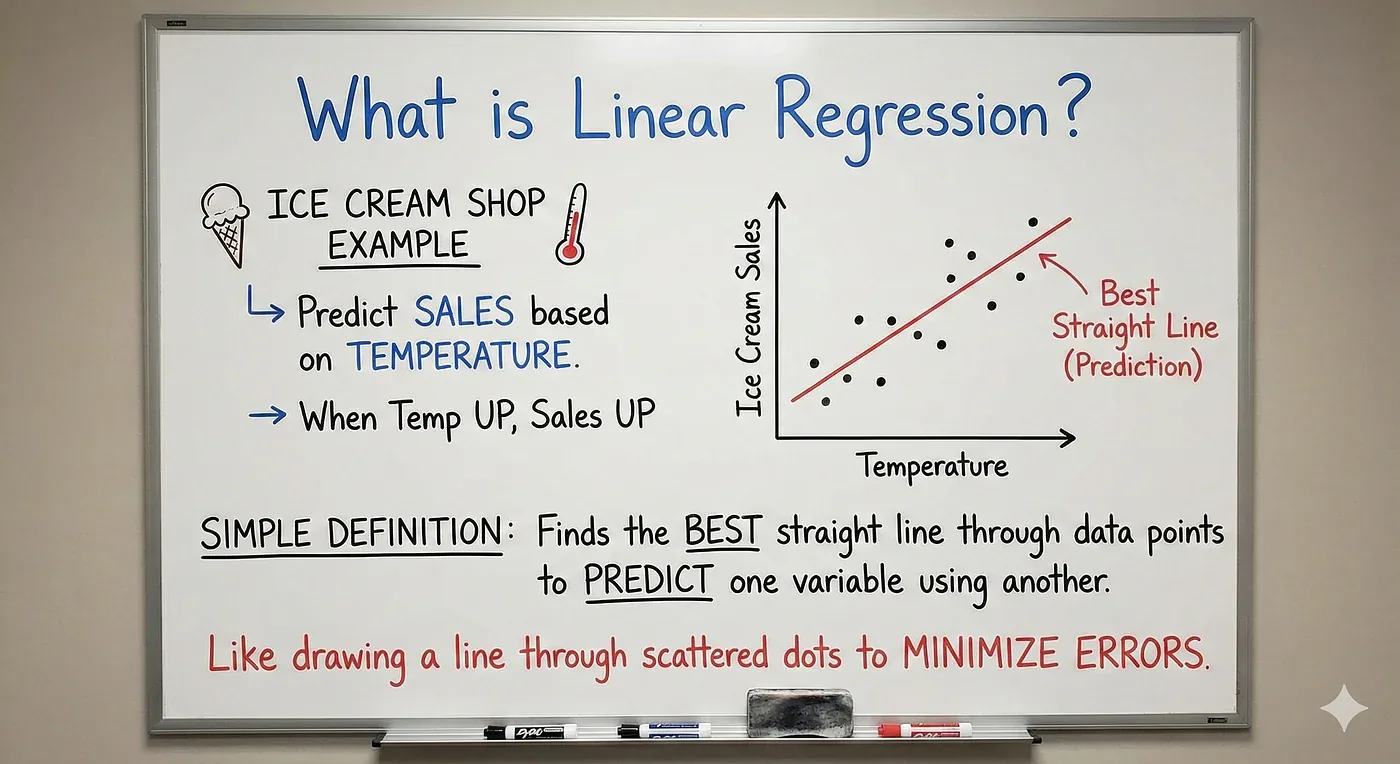
The line is the whole model. Its equation is the one from school, with statisticians' letters:
is what we predict (sales), is the input (temperature). is the intercept, the value of when . is the slope, how much changes when goes up by one. ("epsilon") is the error, everything the line cannot explain. In practice we write the prediction as and keep for the leftover.
With more than one input you simply add more terms, which gives multiple linear regression:
One weight for every feature . With two inputs the "line" is a flat sheet in 3D, with ten inputs it is a flat surface in 11 dimensions that you cannot draw but can still compute with.
Here is the first model in code. The data is made up so that we know the truth, but the noise is realistic.
import numpy as np
import matplotlib.pyplot as plt
from sklearn.linear_model import LinearRegression

# Made-up but realistic: daily temperature (°C) and kulfi sales at a street stall
rng = np.random.default_rng(7)
temp = rng.uniform(22, 44, 40)
sales = 12 * temp - 170 + rng.normal(0, 25, 40)      # a true line plus everyday noise

model = LinearRegression().fit(temp.reshape(-1, 1), sales)
print(f"intercept (b0): {model.intercept_:.1f}")
print(f"slope     (b1): {model.coef_[0]:.2f}  -> each extra degree adds about {model.coef_[0]:.0f} sales")
print(f"prediction for 38 °C: {model.predict([[38]])[0]:.0f} sales")

xs = np.linspace(21, 45, 50)
fig, ax = plt.subplots(figsize=(6.4, 3.8))
ax.scatter(temp, sales, s=22, color="#2563EB", alpha=.75, label="daily sales")
ax.plot(xs, model.predict(xs.reshape(-1, 1)), color="#DC2626", lw=2.2, label="best-fit line")
ax.set_xlabel("temperature (°C)"); ax.set_ylabel("kulfi sold")
ax.legend(frameon=False); ax.spines[["top", "right"]].set_visible(False)
fig.tight_layout()intercept (b0): -217.0
slope (b1): 13.45 -> each extra degree adds about 13 sales
prediction for 38 °C: 294 sales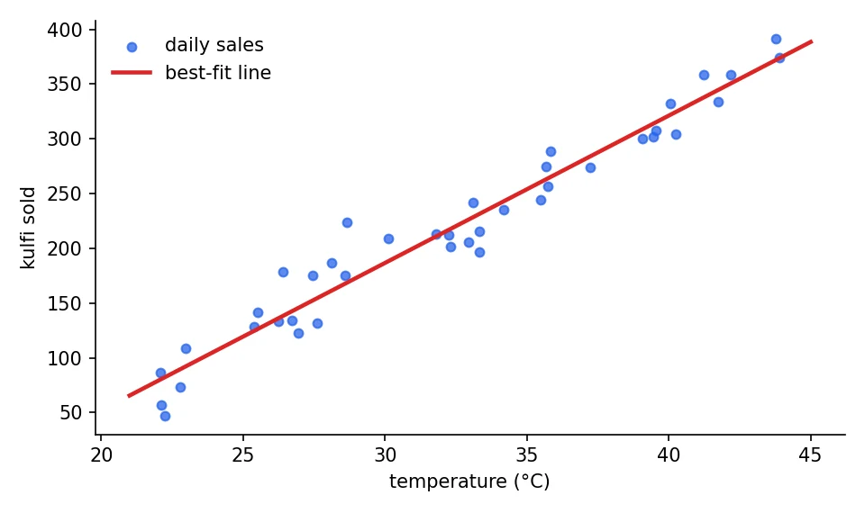
Read the output like a sentence. The intercept says "at 0 °C you would sell about -217", which is nonsense, and that is fine. The intercept only anchors the line, and no one ever sold kulfi at 0 °C, so we should not read meaning into it. The slope says each extra degree adds about 13 sales. The prediction for a 38 °C day is about 294.
A line fitted on 22 to 44 °C says nothing reliable about 5 °C or 60 °C. Predictions inside the range of the training data are interpolation, and that is where regression is trustworthy.
How the best line is found
"Closest to all the dots" needs a definition. For each dot, measure the vertical gap between it and the line (the residual), square it so negatives do not cancel positives, and add them all up. The best line is the one that makes that total as small as possible. That method is called ordinary least squares (OLS).
is the real value, the line's prediction for row . Squaring also punishes big misses much more than small ones, which is why a single wild outlier can drag the line towards itself.
For one input there is a neat closed-form answer. The slope is how much and move together, divided by how much moves on its own:
and are the averages. The second formula says the best line always passes through the point , the centre of the data.
For many inputs, it is easier to write it with matrices. Stack your features into a table (with an extra column of ones for the intercept), and OLS has a one-line solution called the normal equation:
is the transpose of (rows and columns swapped) and is the matrix inverse. In code we use solve instead of explicitly inverting, because it is faster and more numerically stable.
import numpy as np
from sklearn.datasets import load_diabetes
from sklearn.linear_model import LinearRegression

X, y = load_diabetes(return_X_y=True)
A = np.column_stack([np.ones(len(X)), X])            # add a column of 1s for the intercept

beta = np.linalg.solve(A.T @ A, A.T @ y)             # solves (AᵀA) β = Aᵀy
sk = LinearRegression().fit(X, y)

print("intercept  by hand:", round(beta[0], 3), "| scikit-learn:", round(sk.intercept_, 3))
print("bmi weight by hand:", round(beta[3], 3), "| scikit-learn:", round(sk.coef_[2], 3))
print("all weights identical:", np.allclose(beta[1:], sk.coef_))intercept by hand: 152.133 | scikit-learn: 152.133
bmi weight by hand: 519.846 | scikit-learn: 519.846
all weights identical: TrueThat "True" at the bottom is the reassuring bit. LinearRegression is not doing anything mysterious, it is solving the same equation by a more careful route. When we meet neural networks, no such neat formula exists, and that is when gradient descent (Sessions 6 to 8) takes over.
What does the intercept represent in a linear regression?
Real data: ten measurements, one prediction
Back to the diabetes data from Session 1. Now use all ten features at once.
import numpy as np
import pandas as pd
from sklearn.datasets import load_diabetes
from sklearn.linear_model import LinearRegression
from sklearn.model_selection import train_test_split
from sklearn.metrics import r2_score

data = load_diabetes(as_frame=True)
X, y = data.data, data.target
X_tr, X_te, y_tr, y_te = train_test_split(X, y, test_size=0.2, random_state=42)

model = LinearRegression().fit(X_tr, y_tr)
print("R² on training rows:", round(r2_score(y_tr, model.predict(X_tr)), 3))
print("R² on test rows    :", round(r2_score(y_te, model.predict(X_te)), 3))

coefs = pd.Series(model.coef_, index=X.columns).sort_values()
print("\nWeights (sorted):")
print(coefs.round(1).to_string())

print("\ncorrelation between s1 and s2:", round(X["s1"].corr(X["s2"]), 3))R² on training rows: 0.528
R² on test rows : 0.453
Weights (sorted):
s1 -931.5
sex -242.0
age 37.9
s6 48.7
s3 163.4
s4 275.3
bp 347.7
s2 518.1
bmi 542.4
s5 736.2
correlation between s1 and s2: 0.897Three things to read here.
The scores. R² is 0.528 on the training rows and 0.453 on rows the model never saw. The drop is normal, the model is always a little better on data it has studied. A big gap would be a warning sign of overfitting, which is Session 3's problem.
The weights. s5 (a blood-serum reading), bmi (body mass) and bp (blood pressure) are the readable ones, and all push the prediction up, which fits what you would expect medically. sex has a negative weight, but remember these columns were rescaled in the dataset, so a weight is "per unit of a scaled column", not "per mmHg".
The strange pair. Look at s1 (-931) and s2 (+518). Huge, opposite and suspicious. The last line explains it: s1 and s2 are correlated at 0.897, so they carry nearly the same information, and the model can split credit between them in wild ways that cancel out. This is multicollinearity, and it makes individual weights unreliable even when predictions are fine. Ridge and Lasso regression in Session 3 exist largely to tame exactly this.
Measuring the fit: R²
How good is a line? "Accuracy as a percentage" does not make sense for a number. The usual score is R², the coefficient of determination. It asks what fraction of the variation in the model explains, compared with the laziest possible model that always predicts the average.
is the error left after the model, the error of always guessing the mean. is perfect and means no better than the average. On new data it can go below 0, which means the model is worse than guessing the average. Session 4 covers this and the other metrics properly.
When can you trust a linear regression?
OLS gives you a line for any data, whether or not a line is appropriate. The result is only dependable when these conditions roughly hold:
- Linearity. The output really does change in a straight-line way with the inputs.
- Independence. Rows do not influence each other (daily sales on consecutive days often break this).
- Constant spread (homoscedasticity). The size of the errors is about the same everywhere.
- Roughly normal errors. The residuals are bell-shaped. This matters most for confidence intervals, less for plain prediction.
- No strong multicollinearity. Inputs should not be near copies of each other.
You do not have to take these on faith. Two quick plots show most violations:
import matplotlib.pyplot as plt
from scipy import stats
from sklearn.datasets import load_diabetes
from sklearn.linear_model import LinearRegression

X, y = load_diabetes(return_X_y=True)
model = LinearRegression().fit(X, y)
pred = model.predict(X)
resid = y - pred                                      # what the line could not explain

fig, ax = plt.subplots(1, 2, figsize=(10, 3.6))
ax[0].scatter(pred, resid, s=12, alpha=.6, color="#7C3AED")
ax[0].axhline(0, color="#DC2626", lw=1.5)
ax[0].set_xlabel("predicted value"); ax[0].set_ylabel("residual"); ax[0].set_title("Residuals vs predictions")
stats.probplot(resid, dist="norm", plot=ax[1])
ax[1].set_title("Are the residuals bell-shaped?")
ax[1].get_lines()[0].set_markerfacecolor("#2563EB"); ax[1].get_lines()[0].set_markeredgecolor("#2563EB")
for a in ax: a.spines[["top", "right"]].set_visible(False)
fig.tight_layout()
print("mean residual:", round(resid.mean(), 6))mean residual: -0.0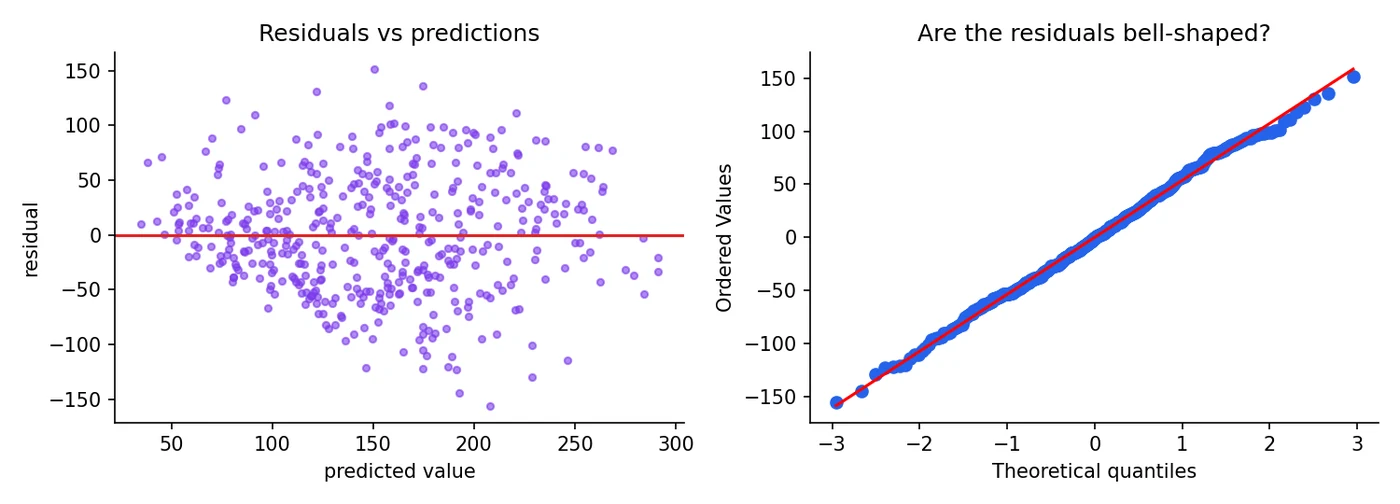
Read the left plot as a doctor reads an X-ray. A healthy picture is a shapeless cloud around the zero line, and that is what we get: no curve, no obvious funnel. A curve would mean the relationship is not linear, a funnel would mean the errors grow with the prediction. In the right plot, dots hugging the red line mean the errors are close to normal, and here they hug it almost the whole way, with only a slight sag at the top right. So the assumptions look fine for this data. Two small pictures told us more about the model's health than a single R² ever could.
When the line is not enough
Real relationships bend. If you force a straight line through a curve, no amount of data helps, the model is simply too stiff. That is underfitting.
import numpy as np
import matplotlib.pyplot as plt
from sklearn.linear_model import LinearRegression
from sklearn.metrics import r2_score
from sklearn.pipeline import make_pipeline
from sklearn.preprocessing import PolynomialFeatures

rng = np.random.default_rng(3)
x = np.sort(rng.uniform(-3, 3, 80))
y = 0.8 * x**2 - x + rng.normal(0, 0.8, 80)           # a curve, not a line
X = x.reshape(-1, 1)

line = LinearRegression().fit(X, y)
curve = make_pipeline(PolynomialFeatures(degree=2), LinearRegression()).fit(X, y)
print("straight line R²  :", round(r2_score(y, line.predict(X)), 3))
print("degree-2 curve R² :", round(r2_score(y, curve.predict(X)), 3))

fig, ax = plt.subplots(figsize=(6.4, 3.8))
ax.scatter(x, y, s=18, color="#2563EB", alpha=.7)
ax.plot(x, line.predict(X), color="#DC2626", lw=2.2, label="straight line")
ax.plot(x, curve.predict(X), color="#16A34A", lw=2.2, label="degree-2 curve")
ax.legend(frameon=False); ax.spines[["top", "right"]].set_visible(False)
fig.tight_layout()straight line R² : 0.427
degree-2 curve R² : 0.909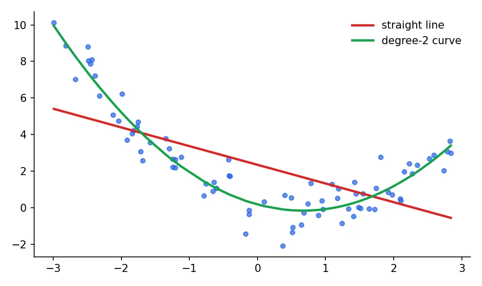
The line explains 43 percent of the variation. Add one extra input, , and it explains 91 percent. Notice that the green curve is still linear regression: it is linear in the weights, we just gave it a squared column to work with. That trick is called polynomial regression. The more flexible a model gets, the more it can also chase noise, which is where Session 3 begins. And when feature-crafting by hand becomes painful, other model families take over: trees (Sessions 11 to 13) and neural networks (Sessions 9, 10 and onwards).
The method of least squares was first published by Adrien-Marie Legendre in 1805. Gauss published his version in 1809 and claimed he had been using it since 1795.history of statistics
The word "regression" comes from Francis Galton, who noticed in the 1880s that very tall parents tended to have children closer to average height: a "regression towards mediocrity".Galton, 1886
Your regression gives R² = 0.91 on the training data but only 0.20 on the test data. What is the most likely problem?
The big picture: from idea to production
Whatever model you use, the journey looks the same: load the data, preprocess it, select features, train, evaluate, export the model, deploy it, and keep monitoring it. Notice that training is only one of eight steps. Most real-world effort goes into the steps around it, and that is also where most bugs hide. A model that is excellent in a notebook and wrong in production is almost always a data problem, not a maths problem.
Try it yourself
- Re-run the kulfi example with
rng = np.random.default_rng(1)and a noise of+ rng.normal(0, 60, 40). How do the slope, the intercept and the plot change? What does that teach you about noise? - Fit a regression on the diabetes data using only
bmi, and compare its test R² with the all-features R² of 0.453. - Drop
s2from the features and refit. What happens to the weight ofs1? - Find two real-world prediction problems around you. Decide whether each is regression or classification, and which columns you would use as inputs.
What comes next
A straight line is simple and fast, and now you can also say precisely when it is not enough. In Session 3 we deal with the thing we just saw: weights that go wild when features overlap, and models that memorise. The fix is regularisation, with two famous flavours called Ridge and Lasso.
Frequently asked questions
What is the difference between AI, machine learning and deep learning?
AI is the broad goal of machines doing tasks that need intelligence. Machine learning is a way of reaching it by learning patterns from data instead of hand-written rules. Deep learning is a type of machine learning that uses many-layered neural networks and learns its own features from raw data. Generative AI is deep learning that creates new text, images or audio.
Is linear regression machine learning or statistics?
Both. Statisticians developed it long before the term machine learning existed, and it is still the standard baseline in ML. What differs is the emphasis: statistics often cares about explaining relationships and confidence intervals, while machine learning cares most about predicting well on unseen data.
What is a good R-squared value?
It depends entirely on the field. Physics experiments can reach 0.99, while predicting human behaviour or health outcomes may be useful at 0.3 to 0.5. Judge R² on test data, compare it with a simple baseline, and never judge it alone. Our diabetes example reaches about 0.45 on unseen patients, which is reasonable for ten simple measurements.
Can linear regression handle curved relationships?
Yes, if you add transformed features such as x squared or the logarithm of x. The model stays linear in its weights even though the fitted curve bends. For very complex patterns, trees or neural networks are usually a better fit.
Do I need to scale features for linear regression?
Plain OLS gives the same predictions whether or not you scale, but scaling makes the weights comparable and is required once you add regularisation or train with gradient descent. It is a good habit to scale inside a pipeline.