Session 6 gave us a number that says how wrong a model is. This session answers the obvious next question: how do you make that number smaller? The answer, gradient descent, is the one algorithm behind almost all of modern machine learning. The model that wrote your autocomplete, the one that recognises faces on your phone and the language models in the news were all trained with some form of it.
The idea fits in one sentence. Look at which way is downhill, take a small step that way, and repeat. We saw it run in the training loop in Session 1 and met its learning rate in Session 5. Here we take it apart properly.
The gradient in plain words
Stand on a hillside in thick fog. You cannot see the valley, but you can feel the ground under your feet. You turn until you find the direction where the ground slopes down most steeply, take a step that way, and feel again. That is gradient descent.
In maths, the gradient is the generalisation of a slope to many dimensions. If the loss depends on many weights, the gradient collects the slope with respect to each weight into a single vector:
is read "nabla" or "del", and is the partial derivative: how much the loss changes when only the weight is nudged. The gradient vector points in the direction of steepest increase, and its length says how steep it is.
The gradient points uphill. We want to go down, so we walk the opposite way:
is the learning rate, the size of each step. This single line is the engine of training. Everything else in this session is a refinement of it.
Here is the smallest working version: minimise , whose slope is and whose lowest point is at .
w, lr = 0.0, 0.1                 # start far from the answer, take small steps

for step in range(51):
    grad = 2 * (w - 3)           # derivative of f(w) = (w - 3)^2
    if step in (0, 1, 2, 5, 10, 25, 50):
        print(f"step {step:2d}   w = {w:.4f}   slope = {grad:7.4f}")
w = w - lr * grad # step AGAINST the slopestep 0 w = 0.0000 slope = -6.0000
step 1 w = 0.6000 slope = -4.8000
step 2 w = 1.0800 slope = -3.8400
step 5 w = 2.0170 slope = -1.9661
step 10 w = 2.6779 slope = -0.6442
step 25 w = 2.9887 slope = -0.0227
step 50 w = 3.0000 slope = -0.0001Look at how the steps shrink. The slope starts at -6 and the weight moves 0.6. The slope falls to -4.8 and the next move is 0.48. By step 25 the slope is almost flat (-0.02) and the weight has all but stopped at 2.9887. By step 50 it sits at 3.0000. The steps get smaller by themselves because the slope gets smaller as we near the bottom. That is a gift: no need to slow down by hand.
Gradient descent was first described by the French mathematician Augustin-Louis Cauchy in 1847, in a paper on solving systems of equations. It is nearly 180 years old and still trains the biggest models today.Cauchy, Comptes Rendus, 1847
Minima: local, global and the shape of the loss
A minimum is a low point of the loss. The global minimum is the lowest point anywhere. A local minimum is only the lowest point in its neighbourhood.
- For linear regression with MSE, the loss is a single smooth bowl. There is exactly one minimum and gradient descent always finds it.
- For neural networks, the loss surface is bumpy: many valleys, long flat regions and "saddle points" that are a minimum in one direction and a maximum in another.
On a bumpy surface the starting point decides where you end up.
import numpy as np
import matplotlib.pyplot as plt

f  = lambda x: x**4 - 3 * x**2 + x          # a bumpy loss with two valleys
df = lambda x: 4 * x**3 - 6 * x + 1         # its slope

def descend(x, lr=0.01, steps=400):
    for _ in range(steps):
        x = x - lr * df(x)
    return x

for start in (-2.0, 2.0):
    end = descend(start)
    print(f"start at x = {start:5.1f}  ->  ends at x = {end:6.3f},  loss = {f(end):7.3f}")

xs = np.linspace(-2.3, 2.3, 400)
fig, ax = plt.subplots(figsize=(6.4, 3.8))
ax.plot(xs, f(xs), color="#111827", lw=2)
for start, col in [(-2.0, "#16A34A"), (2.0, "#DC2626")]:
    end = descend(start)
    ax.scatter([start], [f(start)], color=col, zorder=5); ax.scatter([end], [f(end)], color=col, marker="*", s=180, zorder=5)
ax.set_xlabel("weight"); ax.set_ylabel("loss"); ax.spines[["top", "right"]].set_visible(False)
fig.tight_layout()start at x = -2.0 -> ends at x = -1.301, loss = -3.514
start at x = 2.0 -> ends at x = 1.131, loss = -1.070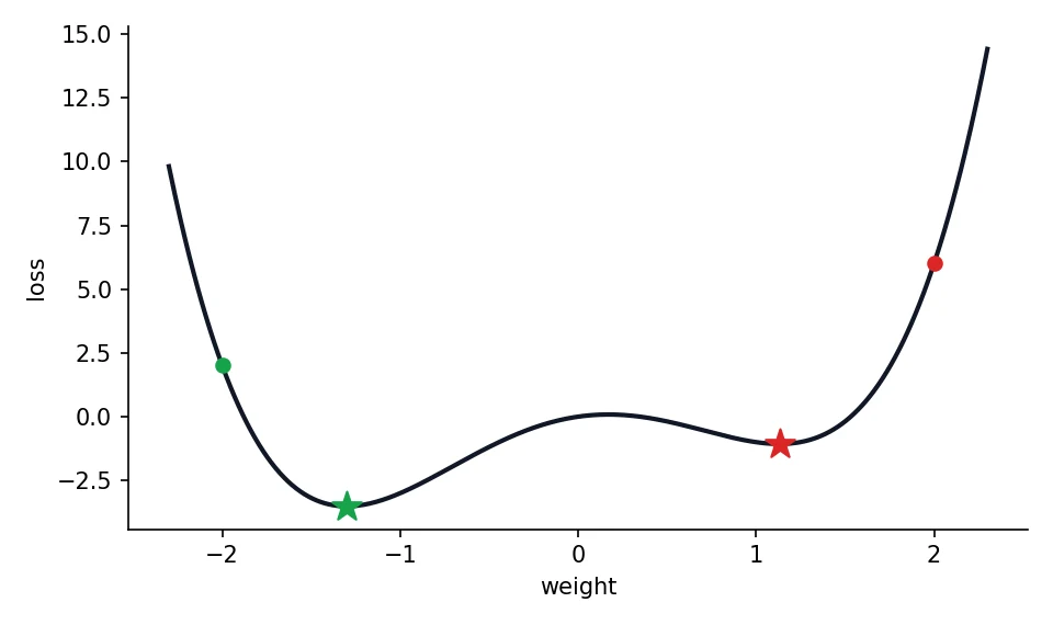
Start at x = -2 and the descent reaches the deeper valley (loss -3.514). Start at x = 2 and it settles into the shallower one (loss -1.070). Same algorithm, same learning rate, different results.
This sounds alarming, and for small problems it is. In practice, large neural networks turn out to be forgiving: most of the local minima they reach are nearly as good as the best one, and the random noise from mini-batches (below) helps shake the model out of poor ones. This is one reason people use random starting weights and train several times.
The three flavours
The only thing that separates the variants is how many rows are used to compute the gradient for one step.
| Batch GD | Stochastic GD (SGD) | Mini-batch GD | |
|---|---|---|---|
| Rows per step | All of them | Exactly 1 | A small group (32, 64, 128) |
| Path | Smooth and direct | Noisy and zig-zagging | Mostly smooth, slightly noisy |
| Cost per step | High (reads everything) | Very low | Low |
| Memory | High | Low | Medium |
| Updates per epoch | 1 | One per row | Rows divided by batch size |
Mini-batch wins in practice. Pure SGD wastes the parallel power of a GPU, which is happiest doing many rows at once, and full batch is too slow and memory-hungry on big data. Mini-batch takes the stability of one and the speed of the other.
import numpy as np
import matplotlib.pyplot as plt
from sklearn.datasets import load_diabetes
from sklearn.preprocessing import StandardScaler

X, y = load_diabetes(return_X_y=True)
X = StandardScaler().fit_transform(X); y = (y - y.mean()) / y.std()
n = len(X)

def run(batch, lr, epochs=25, seed=0):
    rng = np.random.default_rng(seed)
    w = np.zeros(X.shape[1]); curve = []
    for _ in range(epochs):
        order = rng.permutation(n)
        for i in range(0, n, batch):
            idx = order[i:i + batch]
            g = -2 * X[idx].T @ (y[idx] - X[idx] @ w) / len(idx)
            w = w - lr * g
        curve.append(np.mean((y - X @ w) ** 2))
    return np.array(curve)

batch_gd = run(n, 0.1)           # whole dataset: 1 update per epoch
sgd      = run(1, 0.005)         # one row at a time: 442 updates per epoch
mini     = run(32, 0.05)         # mini-batch of 32

for name, c in [("batch", batch_gd), ("SGD (1 row)", sgd), ("mini-batch (32)", mini)]:
    print(f"{name:16s} loss after epoch 1: {c[0]:.3f}   after epoch 25: {c[-1]:.3f}")

fig, ax = plt.subplots(figsize=(6.6, 3.8))
for c, lab, col in [(batch_gd, "batch (all rows)", "#DC2626"), (sgd, "SGD (1 row)", "#F59E0B"), (mini, "mini-batch (32)", "#16A34A")]:
    ax.plot(range(1, 26), c, lw=2, color=col, label=lab)
ax.set_xlabel("epoch"); ax.set_ylabel("loss"); ax.legend(frameon=False); ax.spines[["top", "right"]].set_visible(False)
fig.tight_layout()batch loss after epoch 1: 0.626 after epoch 25: 0.486
SGD (1 row) loss after epoch 1: 0.535 after epoch 25: 0.494
mini-batch (32) loss after epoch 1: 0.503 after epoch 25: 0.486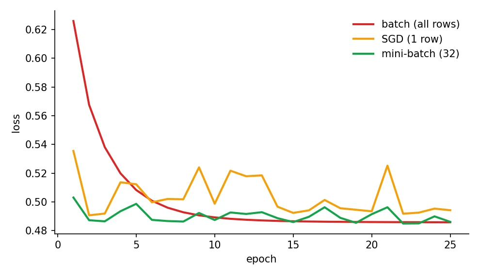
All three end up in the same place (a loss near 0.49), which is the point: they are different routes to the same destination. What differs is the journey. After a single epoch, full-batch GD has made only one step and sits at 0.626. SGD, with 442 steps in that same epoch, is at 0.535, and mini-batch at 0.503. For the same amount of data seen, the variants that update more often get a head start. The learning rates differ because each variant tolerates a different step size: noisy SGD needs a smaller one.
Here is the mini-batch gradient written out, since this is the formula your code uses:
is the set of rows in the current batch and its size. It is an estimate of the true gradient from a small sample, noisy but cheap, and on average it points the right way.
Why is mini-batch gradient descent the standard choice for deep learning?
Beyond plain gradient descent: optimisers
Plain gradient descent has a weakness. On a loss surface shaped like a long narrow valley, the step size is limited by the steep walls (a bigger step would overshoot them and blow up), so progress along the gentle floor is painfully slow. Two ideas fix this, and together they gave us the optimiser most people use by default.
Momentum
Instead of using only the current slope, keep a running memory of recent steps, like a ball with weight that keeps rolling. Steps in a consistent direction pile up speed, and the back-and-forth bouncing cancels out.
is the "velocity" and (often 0.9) controls how much of the past is kept. With this is plain gradient descent.
Adam: a step size per weight
Some weights need big steps and others tiny ones. Adam (Adaptive Moment Estimation) tracks two running averages for every weight: the average gradient (like momentum) and the average squared gradient (a measure of how bumpy that weight's slope is). Then it scales each step by that bumpiness.
is the gradient at step . and are bias-corrected versions of and (they correct for starting at zero). The usual defaults are , and .
The code below compares all three on a deliberately awkward elongated bowl, steep in one direction and gentle in the other.
import numpy as np
import matplotlib.pyplot as plt

# An elongated bowl: very steep in w2, very shallow in w1. Plain gradient descent struggles here.
# (SGD cannot use a bigger step than 2/25 = 0.08 or it blows up in the steep direction.)
A = np.array([1.0, 25.0])
loss = lambda w: 0.5 * (A * w ** 2).sum()
grad = lambda w: A * w

def sgd(lr=0.04, steps=120, w=np.array([4.0, 1.0])):
    path = [w.copy()]
    for _ in range(steps): w = w - lr * grad(w); path.append(w.copy())
    return np.array(path)

def momentum(lr=0.04, beta=0.8, steps=120, w=np.array([4.0, 1.0])):
    v = np.zeros(2); path = [w.copy()]
    for _ in range(steps): v = beta * v + grad(w); w = w - lr * v; path.append(w.copy())
    return np.array(path)

def adam(lr=0.3, b1=0.9, b2=0.999, eps=1e-8, steps=120, w=np.array([4.0, 1.0])):
    m = np.zeros(2); v = np.zeros(2); path = [w.copy()]
    for t in range(1, steps + 1):
        g = grad(w); m = b1 * m + (1 - b1) * g; v = b2 * v + (1 - b2) * g ** 2
        w = w - lr * (m / (1 - b1 ** t)) / (np.sqrt(v / (1 - b2 ** t)) + eps); path.append(w.copy())
    return np.array(path)

paths = {"SGD": sgd(), "SGD + momentum": momentum(), "Adam": adam()}
for name, p in paths.items():
    l = np.array([loss(w) for w in p])
    first = int(np.argmax(l < 1e-3)) if (l < 1e-3).any() else None
    print(f"{name:15s} steps to reach loss < 0.001: {first if first is not None else 'not within 120'}   final loss {l[-1]:.5f}")

gx, gy = np.meshgrid(np.linspace(-1, 4.5, 200), np.linspace(-1.3, 1.3, 200))
fig, ax = plt.subplots(figsize=(7.2, 3.9))
ax.contour(gx, gy, 0.5 * (A[0] * gx ** 2 + A[1] * gy ** 2), levels=12, colors="#CBD5E1", linewidths=1)
for (name, p), c in zip(paths.items(), ["#DC2626", "#F59E0B", "#16A34A"]):
    ax.plot(p[:40, 0], p[:40, 1], "-o", ms=3, lw=1.4, color=c, label=name)
ax.set_xlabel("w1 (gentle slope)"); ax.set_ylabel("w2 (steep slope)"); ax.legend(frameon=False)
ax.spines[["top", "right"]].set_visible(False)
fig.tight_layout()SGD steps to reach loss < 0.001: 111 final loss 0.00044
SGD + momentum steps to reach loss < 0.001: 41 final loss 0.00000
Adam steps to reach loss < 0.001: 61 final loss 0.00004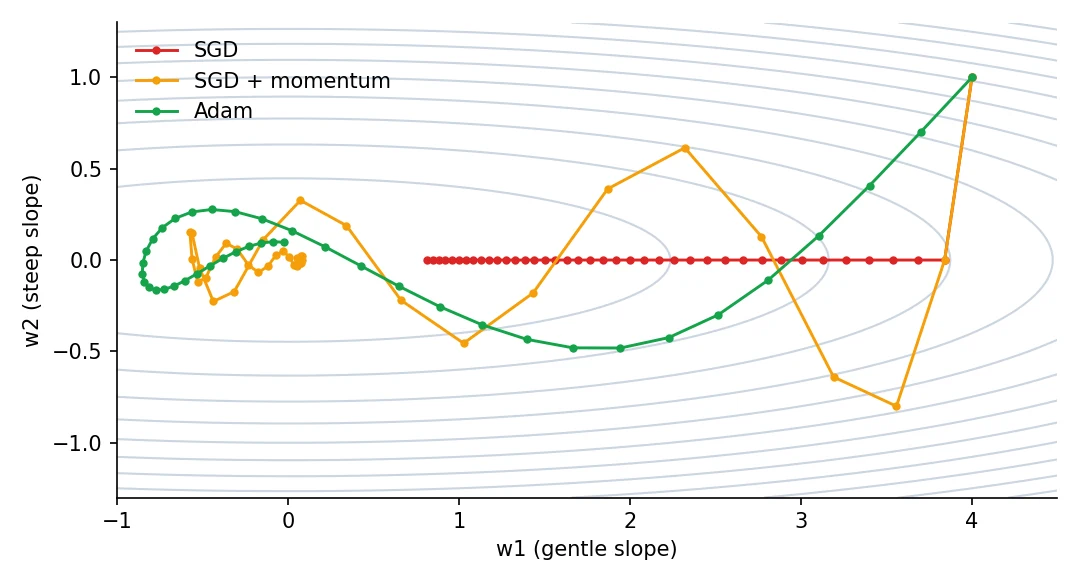
To get below a loss of 0.001, plain SGD needs 111 steps. Momentum needs 41, and Adam 61. The figure shows why. SGD's step is exactly the right size to flatten the steep direction in one move (the red line drops straight onto the axis), and then it can only crawl along the gentle direction at a few percent per step. Momentum and Adam build up speed along that gentle direction instead. One honest caveat: these results depend on the settings, and I picked reasonable ones for each. SGD cannot take a bigger step here without blowing up in the steep direction, which is exactly the limit the others are working around.
Adam was published by Diederik Kingma and Jimmy Ba in 2014 and became the default optimiser for deep learning. Its recommended defaults of 0.001, 0.9 and 0.999 work well on a surprising range of problems.Kingma and Ba, Adam: A Method for Stochastic Optimization, 2014
import torch

# in PyTorch the optimiser does the update step for you
opt = torch.optim.SGD(model.parameters(), lr=0.01, momentum=0.9)
opt = torch.optim.Adam(model.parameters(), lr=1e-3)

# mini-batches come from a DataLoader
# loader = DataLoader(dataset, batch_size=32, shuffle=True)

for xb, yb in loader:
    loss = loss_fn(model(xb), yb)
    opt.zero_grad()      # clear old gradients
    loss.backward()      # backpropagation fills in the new ones (Session 10)
opt.step() # the update ruleopt.zero_grad() clears the old gradients, loss.backward() computes new ones with backpropagation, and opt.step() applies the update. Forget the first one and gradients silently add up across batches.
Choosing an optimiser
| Situation | A good start |
|---|---|
| Quick, reliable default for most neural networks | Adam, lr = 1e-3 |
| You want the best final accuracy on vision models and can tune carefully | SGD with momentum |
| Training Transformers and language models | AdamW (Adam with decoupled weight decay) |
| Tiny convex problems like linear regression | Plain gradient descent or a direct solver |
Try it yourself
- In
gd_scratch.pychange the learning rate to 0.5, then 1.0, then 1.1. What happens at exactly 1.0 and why? (The update becomes .) - In
variants.py, try batch sizes of 8 and 64. Is there a clear best one? - In
local_minima.py, find a starting point between the two valleys where the result flips from one to the other. - In
optimizers.py, raise the SGD learning rate to 0.09 and watch it diverge. What is the safe limit for this surface, and what sets it?
What comes next
Gradient descent works beautifully on shallow models. Stack many layers and a new problem appears: the slopes can shrink to almost nothing by the time they reach the early layers, or blow up. That is Session 8, where we see why, and how learning-rate schedules help the final steps settle.
Frequently asked questions
What is gradient descent in simple terms?
It is a way of finding the lowest point of a loss by repeatedly measuring which direction goes downhill and taking a small step that way. In machine learning, the loss measures how wrong the model is, so going downhill means the model gets better.
What is the difference between batch, stochastic and mini-batch gradient descent?
They differ only in how many rows are used for each step. Batch uses the whole dataset, stochastic uses one row, and mini-batch uses a small group such as 32 or 64. Mini-batch is the standard for deep learning because it is both stable and fast.
What is the learning rate in gradient descent?
It is the size of each step. Too small and training is very slow, too large and the steps overshoot the minimum and the loss can blow up. It is usually the most important hyperparameter to tune.
Is Adam always better than SGD?
No. Adam is a strong default and needs little tuning, but SGD with momentum and a well-chosen schedule sometimes reaches better final accuracy, especially on image models. Many language models use AdamW, a variant of Adam.
Can gradient descent get stuck in a local minimum?
On a bumpy loss surface it can, and where you end up depends on where you start. For large neural networks, most local minima turn out to be nearly as good as the best one, and the noise of mini-batches helps the model escape poor ones.