Everything so far had an answer key. Houses came with prices, tumours came with a diagnosis. But much real data arrives with no labels at all: a shop's customer list, a pile of articles, a log of sensor readings. Nobody can tell you the "right answer" because nobody knows it yet. What you can still ask is, which of these things look alike?
That is clustering, and it is our first taste of unsupervised learning. In the second half of this session we turn to the model that will carry most of the rest of the course, the artificial neural network, and look at its parts before Session 10 opens it up completely. You will want the activation functions from Session 6 and the training idea from Session 7 fresh in your head.
Part A: Clustering
Clustering groups unlabeled points by similarity. "Unsupervised" simply means no one supplied the inputs-and-answers pairs. The algorithm finds structure by itself.
Two flavours of assignment exist. Hard clustering puts every point in exactly one group. Soft (or fuzzy) clustering gives each point a probability for every group, such as 70 percent in group A and 30 percent in group B.
Typical uses: customer segmentation (grouping shoppers for targeted offers), anomaly detection (points that fit no group), and recommendation systems (people who behave alike probably like similar things).
Throughout this part we use a made-up shop with 200 customers, described by their annual income and a spending score from 1 to 100. The helper below generates them, so that you can run everything yourself:
import numpy as np
import pandas as pd

def customers(seed=0):
    """200 made-up shoppers: annual income (thousand rupees) and a 1-100 spending score."""
    rng = np.random.default_rng(seed)
    groups = [(30, 12, 80, 8, 50), (120, 15, 82, 8, 40), (35, 10, 20, 8, 50), (125, 14, 18, 7, 30), (75, 12, 50, 8, 30)]
    rows = []
    for mi, si, ms, ss, n in groups:   # mean income, spread, mean spending, spread, how many
        rows.append(np.column_stack([rng.normal(mi, si, n), rng.normal(ms, ss, n)]))
    X = np.vstack(rows)
    return pd.DataFrame({"income": X[:, 0].clip(5), "spending": X[:, 1].clip(1, 100)}).sample(frac=1, random_state=1).reset_index(drop=True)

df = customers()
We secretly built in five groups of shoppers, but the algorithm will not be told that. The code in the next blocks starts from df = customers().
K-Means: the workhorse
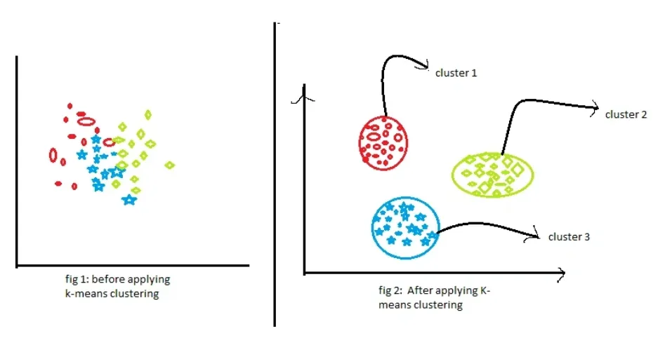
K-Means is the simplest and most used clustering algorithm. You choose , the number of groups. Then it repeats two steps until nothing changes:
- Assign. Give every point to its nearest centre (called a centroid).
- Update. Move each centroid to the average position of the points assigned to it.
It starts from random centres, and after a handful of rounds the centres settle. What it minimises is the total squared distance from each point to its centre:
is the set of points in cluster and its centre (the mean). is the ordinary straight-line (Euclidean) distance. Smaller means tighter groups. scikit-learn calls this number inertia_.
Two rules before you run it. Scale the features first, because K-Means is built on distances and a column measured in thousands would otherwise drown a column measured in tens. And run it several times (n_init=10), since the random start can land it in a poor solution.
import matplotlib.pyplot as plt
from sklearn.cluster import KMeans
from sklearn.preprocessing import StandardScaler

df = customers()
Xs = StandardScaler().fit_transform(df)                    # distances need comparable scales
km = KMeans(n_clusters=5, n_init=10, random_state=0).fit(Xs)
df["segment"] = km.labels_

print(df.groupby("segment").agg(customers=("income", "size"),
                                avg_income=("income", "mean"),
                                avg_spending=("spending", "mean")).round(1))

fig, ax = plt.subplots(1, 2, figsize=(10.5, 3.8), sharex=True, sharey=True)
ax[0].scatter(df["income"], df["spending"], s=16, color="#6B7280"); ax[0].set_title("Before: no labels")
sc = ax[1].scatter(df["income"], df["spending"], s=16, c=df["segment"], cmap="tab10"); ax[1].set_title("After K-Means (k = 5)")
for a in ax: a.set_xlabel("annual income (thousand Rs.)"); a.spines[["top", "right"]].set_visible(False)
ax[0].set_ylabel("spending score")
fig.tight_layout() customers avg_income avg_spending
segment
0 39 121.5 81.6
1 33 75.7 48.9
2 28 123.9 17.0
3 50 31.6 80.3
4 50 35.0 18.6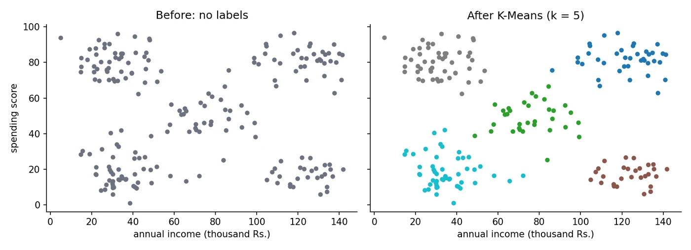
Reading the table is the real work, because the algorithm only gives you numbers 0 to 4. You give them meaning. Segment 0: high income, high spending, the big spenders. Segment 3: low income, high spending, enthusiastic customers on a budget. Segment 2: high income, low spending, people who can afford more but do not shop here (the group a marketing team would target). Segment 4: low income, low spending. Segment 1: the middle of the road. That interpretation, not the clustering itself, is what a business can act on.
How do you choose k?
In real life nobody tells you there are five groups. Two common guides:
- The elbow method. Plot inertia against . It always falls as grows (more centres, shorter distances), so look for the bend where adding another cluster stops paying off.
- The silhouette score. For each point, compare how close it is to its own cluster with how close it is to the nearest other cluster. It runs from -1 to 1, and higher is better.
is the average distance from the point to the others in its own cluster. is the average distance to the points of the nearest other cluster. Near 1 means the point sits comfortably inside its cluster, near 0 means it is on the border, negative means it is probably in the wrong cluster. The score for a clustering is the average over all points.
import matplotlib.pyplot as plt
from sklearn.cluster import KMeans
from sklearn.metrics import silhouette_score
from sklearn.preprocessing import StandardScaler

Xs = StandardScaler().fit_transform(customers())
ks = range(2, 10)
inertia, sil = [], []
for k in ks:
    km = KMeans(n_clusters=k, n_init=10, random_state=0).fit(Xs)
    inertia.append(km.inertia_); sil.append(silhouette_score(Xs, km.labels_))
    print(f"k = {k}   inertia {km.inertia_:7.1f}   silhouette {sil[-1]:.3f}")

fig, ax = plt.subplots(1, 2, figsize=(10, 3.5))
ax[0].plot(list(ks), inertia, "-o", color="#2563EB"); ax[0].set_title("Elbow: inertia vs k")
ax[1].plot(list(ks), sil, "-o", color="#16A34A"); ax[1].set_title("Silhouette score vs k")
for a in ax: a.set_xlabel("number of clusters k"); a.spines[["top", "right"]].set_visible(False)
fig.tight_layout()k = 2 inertia 230.8 silhouette 0.410
k = 3 inertia 131.7 silhouette 0.495
k = 4 inertia 62.5 silhouette 0.601
k = 5 inertia 29.7 silhouette 0.654
k = 6 inertia 26.2 silhouette 0.589
k = 7 inertia 23.5 silhouette 0.504
k = 8 inertia 20.8 silhouette 0.446
k = 9 inertia 18.5 silhouette 0.457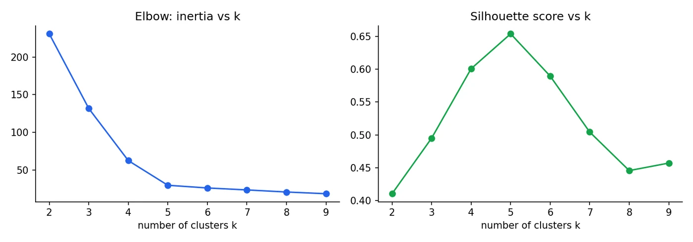
Inertia falls steeply until (62.5 to 29.7) and then crawls (26.2, 23.5, ...), an elbow at 5. The silhouette score peaks at k = 5 with 0.654 and drops after. Both point to the same answer, and that matches the five groups we planted. Real data is rarely this tidy, so treat these as hints, not verdicts.
The standard K-Means algorithm was first proposed by Stuart Lloyd at Bell Labs in 1957, though it was not published until 1982. The name "k-means" was coined by James MacQueen in 1967.Lloyd, 1982; MacQueen, 1967
Why should you scale features before running K-Means?
When K-Means fails: DBSCAN
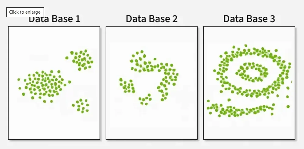
K-Means assumes clusters are round, roughly equal blobs around a centre. Real groups can be curved, stringy or very different in size. DBSCAN (Density-Based Spatial Clustering of Applications with Noise) defines a cluster as a dense region of points that you can walk across without big gaps. It needs no , it follows any shape, and it labels isolated points as noise (label -1). You choose two settings: eps, the neighbourhood radius, and min_samples, how many neighbours make a point "dense".
import numpy as np
import matplotlib.pyplot as plt
from sklearn.cluster import DBSCAN, KMeans
from sklearn.datasets import make_moons
from sklearn.metrics import adjusted_rand_score

X, truth = make_moons(n_samples=400, noise=0.07, random_state=0)
X[:6] += np.random.default_rng(0).uniform(-1.5, 1.5, (6, 2))        # sprinkle in a few outliers

km = KMeans(n_clusters=2, n_init=10, random_state=0).fit_predict(X)
db = DBSCAN(eps=0.2, min_samples=5).fit_predict(X)

print("K-Means agreement with the true shapes:", round(adjusted_rand_score(truth, km), 3))
print("DBSCAN  agreement with the true shapes:", round(adjusted_rand_score(truth, db), 3))
print("DBSCAN clusters found:", len(set(db)) - (1 if -1 in db else 0), "| points labelled noise:", int((db == -1).sum()))

fig, ax = plt.subplots(1, 2, figsize=(9.5, 3.6), sharex=True, sharey=True)
ax[0].scatter(X[:, 0], X[:, 1], c=km, cmap="coolwarm", s=14); ax[0].set_title("K-Means cuts it in half")
ax[1].scatter(X[:, 0], X[:, 1], c=np.where(db == -1, 2, db), cmap="viridis", s=14); ax[1].set_title("DBSCAN follows the shape (noise = yellow)")
for a in ax: a.spines[["top", "right"]].set_visible(False)
fig.tight_layout()K-Means agreement with the true shapes: 0.269
DBSCAN agreement with the true shapes: 0.96
DBSCAN clusters found: 2 | points labelled noise: 2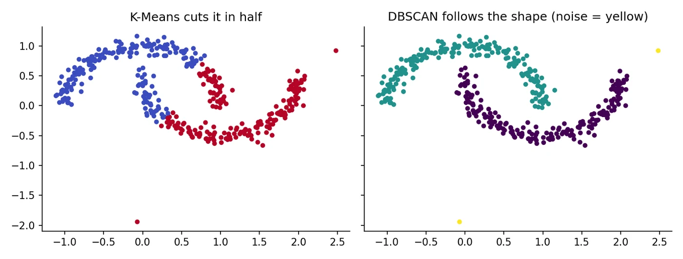
On two curved "moons", K-Means scores only 0.269 against the truth (1.0 is perfect), because it cuts the plane with a straight line between two centres. DBSCAN scores 0.96, finds exactly two clusters, and tags 2 stray points as noise. Always plot your clusters, because a bad clustering still produces tidy-looking numbers.
Hierarchical clustering and soft clustering
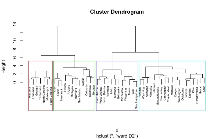
Hierarchical (agglomerative) clustering starts with every point as its own cluster and repeatedly merges the two closest groups, building a tree. You get a whole family of clusterings at once, and you pick one by cutting the tree.
import matplotlib.pyplot as plt
from scipy.cluster.hierarchy import dendrogram, linkage
from sklearn.preprocessing import StandardScaler

Xs = StandardScaler().fit_transform(customers().head(40))      # a small sample keeps the tree readable
Z = linkage(Xs, method="ward")                                  # repeatedly merge the two closest groups

fig, ax = plt.subplots(figsize=(9, 3.6))
dendrogram(Z, ax=ax, no_labels=True, color_threshold=4.5, above_threshold_color="#9CA3AF")
ax.set_ylabel("distance when merged"); ax.spines[["top", "right"]].set_visible(False)
fig.tight_layout()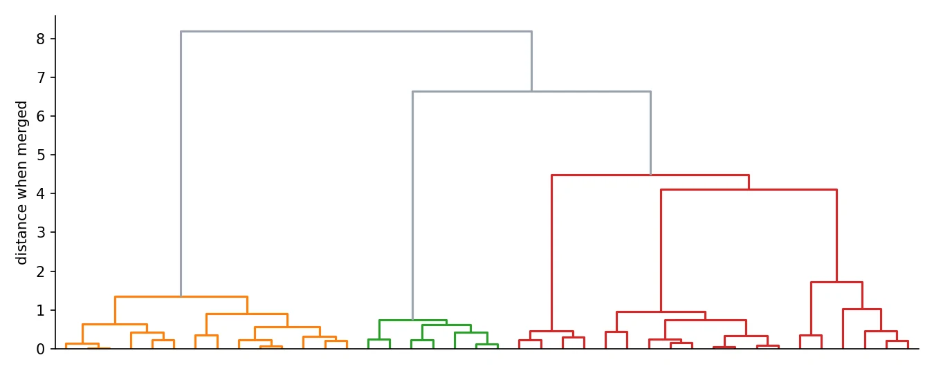
The fourth family, distribution-based clustering, assumes the data came from a mix of bell-shaped (Gaussian) distributions. A Gaussian mixture model (GMM) fits that mixture and gives every point a probability of belonging to each group, which is soft clustering.
import numpy as np
from sklearn.mixture import GaussianMixture
from sklearn.preprocessing import StandardScaler

Xs = StandardScaler().fit_transform(customers())
gmm = GaussianMixture(n_components=5, random_state=0).fit(Xs)
probs = gmm.predict_proba(Xs)

hard = probs.max(axis=1)
i = int(np.argsort(hard)[5])                                   # a customer sitting between groups
print("one borderline customer, membership by cluster:", probs[i].round(2))
print("share of customers the model is <90% sure about:", f"{(hard < 0.9).mean():.0%}")one borderline customer, membership by cluster: [0. 0.05 0. 0.95 0. ]
share of customers the model is <90% sure about: 2%Here a borderline customer is 95 percent in one group and 5 percent in another. Most customers are over 90 percent sure, since our groups are well separated. On messier data you would see many more shared memberships.
| Type | Algorithm | Needs k? | Handles odd shapes? | Finds outliers? |
|---|---|---|---|---|
| Centroid | K-Means | Yes | No (round blobs) | No |
| Density | DBSCAN | No | Yes | Yes (as noise) |
| Hierarchical | Agglomerative | Choose when you cut | Depends on linkage | Not directly |
| Distribution | Gaussian mixture | Yes | Elliptical blobs | By low probability |
from sklearn.cluster import KMeans, DBSCAN, AgglomerativeClustering
from sklearn.preprocessing import StandardScaler

Xs = StandardScaler().fit_transform(X)
km_labels = KMeans(n_clusters=3, n_init=10, random_state=0).fit_predict(Xs)
db_labels = DBSCAN(eps=0.5, min_samples=5).fit_predict(Xs)               # -1 = noise
hc_labels = AgglomerativeClustering(n_clusters=3, linkage="ward").fit_predict(Xs)
Part B: Artificial neural networks
Time to meet the model that dominates the rest of this course. An artificial neural network (ANN) is a function built from many small units called neurons, loosely inspired by the brain, arranged in layers. Each neuron does something very small. The network as a whole can learn remarkably complicated patterns.
You have already met the single neuron in Session 6: a weighted sum followed by an activation function. A layer is just many neurons side by side, and a network is layers stacked one after another.
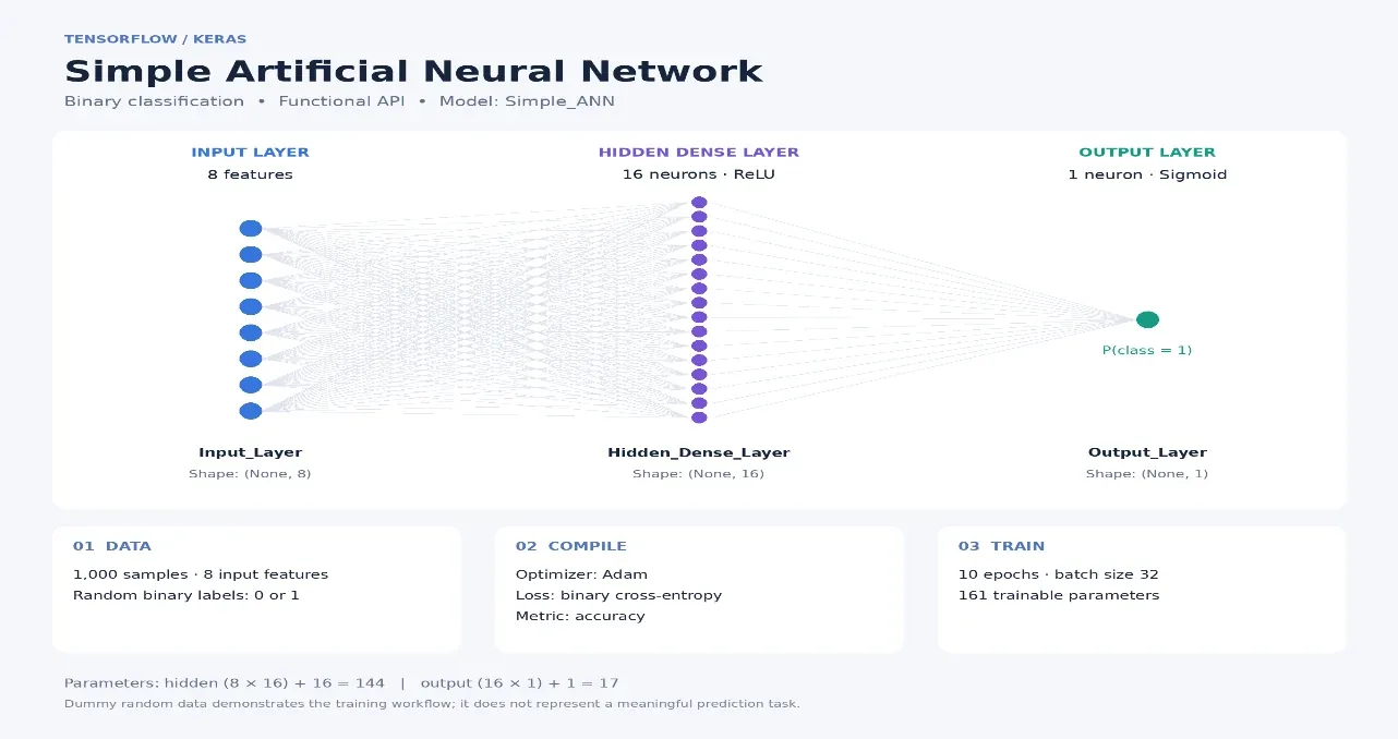
The building blocks
- Input layer. Receives the numbers. It does no computing, it just holds the features.
- Hidden layers. The trainable middle. Each learns to detect patterns, and later layers combine earlier ones into more complex ideas.
- Output layer. Produces the answer: a number for regression, a probability (sigmoid) for yes/no, or a probability per class (softmax).
- Weights and biases. The learned parameters. One weight on every connection, one bias per neuron.
- Activation function. The bend that makes depth worthwhile (Session 6).
All the neurons of one layer can be computed at once with a matrix multiplication:
is the layer number, the previous layer's outputs, the matrix of weights (one row per neuron) and the biases. The output feeds the next layer. This is forward propagation.
The recipe for learning is the same one from Session 1: forward pass, loss, backpropagation to find how every weight contributed to the error, and an optimiser (SGD, Adam) to update. Session 10 shows backprop with every number visible. Here is the 8-16-1 network from the figure, trained for 100 epochs on a made-up binary classification problem with 8 features:
import torch
import torch.nn as nn
from sklearn.datasets import make_classification
from sklearn.model_selection import train_test_split
from sklearn.preprocessing import StandardScaler

torch.manual_seed(0)
X, y = make_classification(n_samples=1000, n_features=8, n_informative=5, random_state=0)
X = StandardScaler().fit_transform(X)
X_tr, X_te, y_tr, y_te = train_test_split(X, y, test_size=0.25, random_state=0)
X_tr, X_te = torch.tensor(X_tr, dtype=torch.float32), torch.tensor(X_te, dtype=torch.float32)
y_tr, y_te = torch.tensor(y_tr, dtype=torch.float32).view(-1, 1), torch.tensor(y_te, dtype=torch.float32).view(-1, 1)

net = nn.Sequential(
    nn.Linear(8, 16),    # input layer (8 features) -> hidden layer (16 neurons)
    nn.ReLU(),
    nn.Linear(16, 1),    # hidden -> output (1 neuron)
    nn.Sigmoid(),        # probability for binary classification
)
print(net)
print("trainable parameters:", sum(p.numel() for p in net.parameters()))   # (8*16+16) + (16*1+1)

opt = torch.optim.Adam(net.parameters(), lr=0.01)
loss_fn = nn.BCELoss()
for epoch in range(1, 101):
    loss = loss_fn(net(X_tr), y_tr)
    opt.zero_grad(); loss.backward(); opt.step()
    if epoch in (1, 10, 50, 100):
        print(f"epoch {epoch:3d}   loss {loss.item():.3f}")

with torch.no_grad():
    acc = ((net(X_te) > 0.5).float() == y_te).float().mean().item()
print(f"test accuracy: {acc:.3f}")Sequential(
(0): Linear(in_features=8, out_features=16, bias=True)
(1): ReLU()
(2): Linear(in_features=16, out_features=1, bias=True)
(3): Sigmoid()
)
trainable parameters: 161
epoch 1 loss 0.719
epoch 10 loss 0.544
epoch 50 loss 0.188
epoch 100 loss 0.092
test accuracy: 0.956Look at the printout. The model has 161 parameters: the hidden layer has and the output layer . The loss falls from 0.719 to 0.092 and the test accuracy lands at 0.956 on 250 rows the network never saw.
The human brain has about 86 billion neurons. Our network above has just 17 working neurons. Even so, the learning recipe is closely related to the one that trains networks with hundreds of billions of parameters.Azevedo et al., Journal of Comparative Neurology, 2009
Types of networks
The one above is a feedforward neural network (FNN): information flows strictly one way, input to output. Two specialised families branch off it, and they are the subjects of Part IV:
- Convolutional neural networks (CNNs) for images and other grid-like data. They slide small filters across the input (Session 16).
- Recurrent neural networks (RNNs) for sequences such as text or prices. They keep a memory of earlier steps (Session 18).
Both, and the Transformer that later replaced RNNs for language, grow out of the same parts you just met.
Clustering and neural networks are the two "unlabelled" and "stacked layers" ideas that look unrelated. They meet again later: a neural network's hidden layers learn representations, and you can cluster those representations too. Embeddings in Session 22 do exactly that.
A network has 10 inputs, one hidden layer of 20 neurons, and 1 output neuron. How many parameters does it have?
Try it yourself
- Change the number of clusters in
kmeans_segments.pyto 3 and then 7. How do the segment averages change? Which would you actually give to a marketing team? - In
dbscan_vs_kmeans.py, tryepsvalues of 0.1 and 0.5. What happens to the number of clusters and the noise points? - Change
ann_basics.pyto have 4 hidden neurons instead of 16. How many parameters now? Does accuracy drop? - Replace the ReLU in the ANN with
nn.Sigmoid(). Does it train as quickly?
What comes next
We have seen the parts of a neural network and watched one train, but the forward and backward passes happened inside loss.backward(). In Session 10 we build a network from nothing but NumPy, compute every number by hand and finally see backpropagation, the algorithm that made deep learning possible.
Frequently asked questions
What is the difference between supervised and unsupervised learning?
Supervised learning trains on examples that come with the right answer, such as house prices or diagnoses. Unsupervised learning has no answers and tries to find structure on its own, for example by grouping similar customers. Clustering is the best-known unsupervised task.
How do I choose the number of clusters in K-Means?
Use the elbow method (look for the bend in the inertia curve) and the silhouette score (pick the k with the highest value), and then check whether the segments make sense for your problem. Both are guides, not proofs, and domain knowledge should have the last word.
When should I use DBSCAN instead of K-Means?
When clusters are not round, differ a lot in size, or the data has outliers you want to flag. DBSCAN follows dense regions of any shape and marks isolated points as noise. K-Means is faster and simpler when groups really are compact blobs.
What is a neuron in a neural network?
A neuron computes a weighted sum of its inputs plus a bias, and passes the result through an activation function such as ReLU. A layer is a group of neurons, and a network is several layers stacked.
What is the difference between parameters and activations in a neural network?
Parameters (weights and biases) are the learned values stored in the model. They change during training and stay fixed when the model makes predictions. Activations are the outputs the neurons compute for each input as it flows through. They are recomputed every time and are not stored.