Random Forest Explained: Bagging, Out-of-Bag Score and Feature Importance

In 1906, around 800 visitors at a country fair in England tried to guess the weight of an ox. Most guesses were wildly off. But the statistician Francis Galton later worked out that the median of the crowd's guesses landed within about one percent of the true weight. Many noisy opinions, averaged, beat almost any single one.

A random forest is that idea applied to the decision trees of Session 11. One tree is unstable and overfits. A few hundred trees, each a bit different and each allowed to be wrong in its own way, vote together and the mistakes cancel out. This session shows how the forest is built, why it works, and what it can and cannot do, with real output you can reproduce.

The two sources of randomness

A forest takes a high-variance model (a deep tree) and makes many different versions of it. Two ingredients do the work.

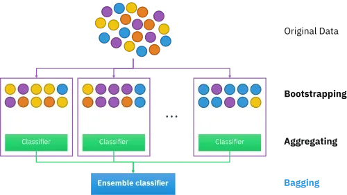
1. Bootstrapping: random rows. Each tree trains on its own sample of the training data, drawn with replacement. Drawing with replacement means a row can be picked several times and some rows are not picked at all. If the data has $n$ rows, each tree's sample also has $n$ rows.

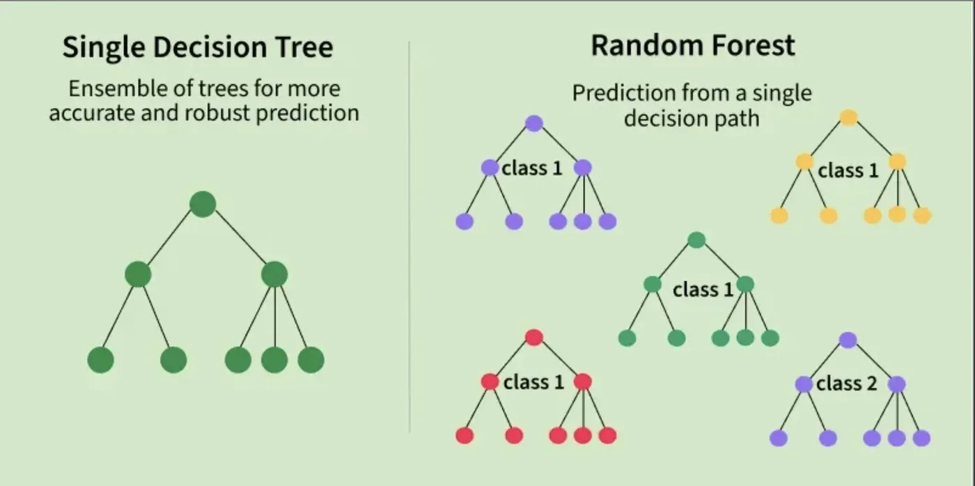
2. Feature randomness: random columns. At every split, the tree is only allowed to look at a random subset of the features (often $\sqrt{p}$ of $p$ features) instead of all of them. This stops one strong feature from dominating every tree, so the trees stay different from each other.

Then the aggregation: every tree predicts independently, and the forest takes a majority vote for classification or the average for regression.

The first two steps together, sampling rows with replacement and then aggregating, are called bagging (bootstrap aggregating). They are two separate steps, so keep them apart in your head: bootstrapping makes the datasets, aggregating combines the answers.

How much data does each tree actually see?

A neat fact about sampling with replacement. If you draw $n$ times from $n$ rows, how many different rows end up in the sample? Each row has a $1 - (1 - 1/n)^n$ chance of being picked at least once, which tends to $1 - 1/e$ as $n$ grows.

import numpy as np

rng = np.random.default_rng(0)
n = 1000
unique_share = []
for _ in range(200):
    sample = rng.integers(0, n, size=n)          # draw n rows WITH replacement
    unique_share.append(len(np.unique(sample)) / n)

print(f"average share of distinct rows in one bootstrap sample: {np.mean(unique_share):.3f}")
print(f"share left out ('out-of-bag'):                          {1 - np.mean(unique_share):.3f}")
print(f"the maths says 1 - 1/e = {1 - 1 / np.e:.3f}")

average share of distinct rows in one bootstrap sample: 0.633
share left out ('out-of-bag'):                          0.367
the maths says 1 - 1/e = 0.632

The simulation gives 0.633, matching the formula's 0.632. That leftover 36.8 percent is a gift: every tree has rows it never trained on, so we can test it on them. Collect those predictions across the forest and you get the out-of-bag score, a free estimate of test accuracy with no separate test set needed.

Why averaging helps: the maths in one line

Suppose each tree's prediction has variance $\sigma^2$ and any two trees are correlated by $\rho$. The variance of the average of $B$ trees is:

This also tells you what a forest cannot do. If every tree makes the same mistake (all high $\rho$, or a systematic bias), averaging does not remove it. That is the job of boosting, in Session 13.

A forest against a single tree

Same breast-cancer data as last session. To avoid being fooled by one lucky split, the comparison uses 20 different train/test splits (5 folds repeated 4 times).

import numpy as np
from sklearn.datasets import load_breast_cancer
from sklearn.ensemble import RandomForestClassifier
from sklearn.model_selection import RepeatedStratifiedKFold, cross_val_score
from sklearn.tree import DecisionTreeClassifier

X, y = load_breast_cancer(return_X_y=True)
cv = RepeatedStratifiedKFold(n_splits=5, n_repeats=4, random_state=0)      # 20 different train/test splits

models = {"one decision tree": DecisionTreeClassifier(random_state=0),
          "random forest (200 trees)": RandomForestClassifier(n_estimators=200, random_state=0, n_jobs=-1)}
for name, m in models.items():
    s = cross_val_score(m, X, y, cv=cv)
    print(f"{name:27s} mean accuracy {s.mean():.3f}   spread (std) {s.std():.3f}   worst split {s.min():.3f}")

rf = RandomForestClassifier(n_estimators=200, oob_score=True, random_state=0, n_jobs=-1).fit(X, y)
print(f"\nout-of-bag accuracy of the forest (free, no test set needed): {rf.oob_score_:.3f}")

one decision tree           mean accuracy 0.926   spread (std) 0.019   worst split 0.886
random forest (200 trees)   mean accuracy 0.963   spread (std) 0.019   worst split 0.904

out-of-bag accuracy of the forest (free, no test set needed): 0.965

A single tree averages 92.6 percent. The forest averages 96.3 percent, a jump of nearly four points from a change of one line of code. One honest observation: the spread across splits is identical (0.019) for both, because most of that spread comes from which patients happen to land in the test set. The forest's gain is in the average, not in being steadier from split to split.

The bottom line is the OOB accuracy, 0.965, calculated from rows each tree never saw. It lands within a fraction of a point of the cross-validated 0.963, which is the proof that it really is a trustworthy free estimate.

How many trees?

More trees is not a hyperparameter you need to agonise over. Unlike tree depth, more trees will not overfit: they only stop helping.

import numpy as np
import matplotlib.pyplot as plt
from sklearn.datasets import load_breast_cancer
from sklearn.ensemble import RandomForestClassifier

X, y = load_breast_cancer(return_X_y=True)
counts = [1, 2, 3, 5, 10, 20, 40, 80, 150, 300]
oob_err = []
for n in counts:
    rf = RandomForestClassifier(n_estimators=n, oob_score=True, bootstrap=True, random_state=0, n_jobs=-1).fit(X, y)
    oob_err.append(1 - rf.oob_score_ if n > 5 else np.nan)       # a handful of trees leaves some rows never out-of-bag
    print(f"{n:4d} trees   out-of-bag accuracy {rf.oob_score_:.3f}")

fig, ax = plt.subplots(figsize=(6.2, 3.6))
ax.semilogx(counts, [1 - e if not np.isnan(e) else np.nan for e in oob_err], "-o", ms=4, lw=2, color="#0D9488")
ax.set_xlabel("number of trees"); ax.set_ylabel("out-of-bag accuracy"); ax.spines[["top", "right"]].set_visible(False)
fig.tight_layout()

   1 trees   out-of-bag accuracy 0.566
   2 trees   out-of-bag accuracy 0.696
   3 trees   out-of-bag accuracy 0.784
   5 trees   out-of-bag accuracy 0.866
  10 trees   out-of-bag accuracy 0.935
  20 trees   out-of-bag accuracy 0.961
  40 trees   out-of-bag accuracy 0.967
  80 trees   out-of-bag accuracy 0.968
 150 trees   out-of-bag accuracy 0.967
 300 trees   out-of-bag accuracy 0.965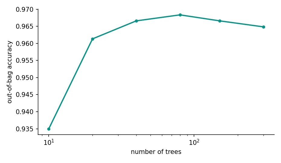

With 1 to 3 trees the score is poor (and the very first values are especially unreliable, since with so few trees many rows are never out-of-bag). By 20 trees it has reached 0.961, and from 40 to 300 it stays within a hair of 0.967. A few hundred trees is plenty. Past that you only pay in time and memory.

Feature importance, and why to be careful

A forest can tell you which columns it relied on. The default measure, impurity importance, adds up how much each feature reduced impurity across all splits in all trees.

import numpy as np
import matplotlib.pyplot as plt
from sklearn.datasets import load_breast_cancer
from sklearn.ensemble import RandomForestClassifier
from sklearn.inspection import permutation_importance
from sklearn.model_selection import train_test_split

data = load_breast_cancer()
X_tr, X_te, y_tr, y_te = train_test_split(data.data, data.target, test_size=0.3, random_state=3, stratify=data.target)
rf = RandomForestClassifier(n_estimators=300, random_state=0, n_jobs=-1).fit(X_tr, y_tr)
print("test accuracy:", round(rf.score(X_te, y_te), 3))

imp = rf.feature_importances_
perm = permutation_importance(rf, X_te, y_te, n_repeats=20, random_state=0).importances_mean
top = np.argsort(imp)[::-1][:8]
print("\n   feature                  impurity   permutation")
for i in top:
    print(f"   {data.feature_names[i]:24s} {imp[i]:.3f}      {perm[i]:.3f}")

fig, ax = plt.subplots(figsize=(6.6, 3.8))
ax.barh([data.feature_names[i] for i in top][::-1], imp[top][::-1], color="#0D9488")
ax.set_xlabel("importance (share of the forest's splitting power)"); ax.spines[["top", "right"]].set_visible(False)
fig.tight_layout()

test accuracy: 0.971

   feature                  impurity   permutation
   worst concave points     0.142      0.002
   worst perimeter          0.126      0.001
   worst radius             0.115      0.005
   worst area               0.104      0.005
   mean concave points      0.095      0.001
   mean concavity           0.057      -0.003
   mean perimeter           0.054      -0.005
   mean radius              0.039      -0.002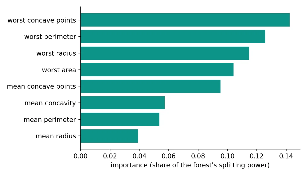

The forest leans on size and shape measures such as worst concave points, worst perimeter, worst radius and worst area. But look at the second column, permutation importance, which shuffles one feature and measures how much the test accuracy drops. It is close to zero for all of them. That is not a contradiction, it is a warning. These features are strongly correlated (perimeter, radius and area all describe size), so when you scramble one, the others carry the information and accuracy barely moves. Impurity importance spreads credit across correlated features, and permutation importance can show none of them as essential. Neither is "wrong". They answer slightly different questions, so check both before telling anyone which feature "matters most".

The bagging family

Random forest is one member of a family:

• Bagged decision trees: bootstrap rows only, all features available at every split.
• Random forest: bootstrap rows and random features at each split.
• Extra Trees (extremely randomised trees): also pick the split thresholds at random instead of searching for the best one. Faster, and a little more variance reduction at a small cost in bias.
• Random subspace: sample only columns, not rows.

from sklearn.datasets import load_breast_cancer
from sklearn.ensemble import BaggingClassifier, ExtraTreesClassifier, RandomForestClassifier
from sklearn.model_selection import RepeatedStratifiedKFold, cross_val_score
from sklearn.tree import DecisionTreeClassifier

X, y = load_breast_cancer(return_X_y=True)
cv = RepeatedStratifiedKFold(n_splits=5, n_repeats=4, random_state=0)
models = {
    "single tree":                DecisionTreeClassifier(random_state=0),
    "bagged trees (50)":          BaggingClassifier(estimator=DecisionTreeClassifier(), n_estimators=50, max_samples=0.8, random_state=0),
    "random forest (200)":        RandomForestClassifier(n_estimators=200, random_state=0, n_jobs=-1),
    "extra trees (200)":          ExtraTreesClassifier(n_estimators=200, random_state=0, n_jobs=-1),
}
for name, m in models.items():
    s = cross_val_score(m, X, y, cv=cv)
    print(f"{name:22s} accuracy {s.mean():.3f}  (+/- {s.std():.3f})")

single tree            accuracy 0.926  (+/- 0.019)
bagged trees (50)      accuracy 0.954  (+/- 0.020)
random forest (200)    accuracy 0.963  (+/- 0.019)
extra trees (200)      accuracy 0.967  (+/- 0.018)

Each step of added randomness helps a little here: a single tree 92.6 percent, bagged trees 95.4, a random forest 96.3 and Extra Trees 96.7. The differences between the last two are small enough that they are within the noise on a dataset this size, so choose by speed and by what suits your data.

from sklearn.ensemble import RandomForestClassifier, BaggingClassifier, ExtraTreesClassifier
from sklearn.tree import DecisionTreeClassifier

rf = RandomForestClassifier(n_estimators=200, max_depth=None, max_features="sqrt",
                            oob_score=True, n_jobs=-1, random_state=0)
rf.fit(X_train, y_train)
print(rf.oob_score_)                  # accuracy on out-of-bag samples
print(rf.feature_importances_)        # which columns mattered most

bag = BaggingClassifier(estimator=DecisionTreeClassifier(), n_estimators=50,
                        max_samples=0.8, bootstrap=True, random_state=0)
extra = ExtraTreesClassifier(n_estimators=200, random_state=0)

n_estimators is the number of trees, max_features the random columns tried at each split, and oob_score=True gives the free estimate. Use RandomForestRegressor when the target is a number.

Forests for numbers

Forests also do regression, averaging the trees' numeric outputs. On the Part I diabetes data:

from sklearn.datasets import load_diabetes
from sklearn.ensemble import RandomForestRegressor
from sklearn.linear_model import LinearRegression
from sklearn.metrics import mean_squared_error, r2_score
from sklearn.model_selection import train_test_split

X, y = load_diabetes(return_X_y=True)
X_tr, X_te, y_tr, y_te = train_test_split(X, y, test_size=0.2, random_state=42)

for name, m in [("linear regression", LinearRegression()),
                ("random forest (300 trees, depth 4)", RandomForestRegressor(n_estimators=300, max_depth=4, random_state=0))]:
    pred = m.fit(X_tr, y_tr).predict(X_te)
    print(f"{name:36s} test R² {r2_score(y_te, pred):.3f}   MSE {mean_squared_error(y_te, pred):7.1f}")

linear regression                    test R² 0.453   MSE  2900.2
random forest (300 trees, depth 4)   test R² 0.476   MSE  2778.7

The forest reaches a test R² of 0.476 against the linear model's 0.453. It is a modest gain, and a useful reminder that a forest is not automatically a miracle. Ten simple measurements on 442 patients are close to linear already, so there is little non-linear structure to find. Forests earn their keep on tables with interactions and odd shapes.

When a forest is the wrong tool

• A systematic mistake. If all trees share the same bias, averaging keeps it. Boosting targets bias directly.
• Size and speed. Hundreds of deep trees take memory, and predictions are slower than a single tree or a linear model.
• Interpretability. You lose the single readable flowchart. Feature importance helps but is not the same.
• Extrapolation. Like a tree, a forest cannot predict beyond the range of values it saw in training.
• Missing values. Many implementations still expect you to fill them in first, though newer versions of scikit-learn have added limited support.

Try it yourself

1. In forest_vs_tree.py, set max_depth=3 for the forest. Does the cross-validated accuracy go up or down?
2. In n_trees.py, change max_features="sqrt" to max_features=None (all features). How does accuracy at 20 trees change? Why does it make the trees more similar?
3. Compute permutation importance on the training set instead of the test set. Do the numbers change?
4. Fit a forest on the diabetes data with max_depth=None. Does R² go up or fall?

What comes next

A forest averages trees that are trained independently, so it cuts variance. But if the underlying trees are too simple, or all miss the same pattern, the average inherits the error. Session 13 takes a different approach: build the trees one after another, each one specialising in what the previous ones got wrong.

Frequently asked questions