Part I ended with a model that can learn a line, be scored and be tuned. Part II opens the engine room. How does a model actually improve? It needs two things before anything else. First, a number that says how wrong it currently is. Second, a way to bend its output so it can learn more than a straight line.
Those two things are the loss function and the activation function. They look like small details. They are not. Pick the wrong loss and your model optimises something you did not care about. Pick the wrong activation and a deep network can stop learning entirely, which is the subject of Session 8. Everything here builds on the training loop you ran in Session 1 and the hyperparameters from Session 5.
Loss versus cost
The two words get used loosely, so here is the usual split.
- A loss function measures the error on one training example.
- A cost function averages those losses over the whole dataset (or a batch). It is the single number gradient descent tries to push down.
In practice people say "loss" for both, and so will this course, but the difference is worth knowing when you read papers. During the forward pass the model makes a prediction and the loss says how wrong it was. Then the backward pass uses that number to decide how every weight should change.
The right loss depends on the output. Numbers need regression losses. Categories need classification losses.
Losses for regression
Mean squared error (MSE, or L2 loss)
You have used this one since Session 1. It squares each error, so big mistakes count far more than small ones.
Smooth and easy to differentiate, which is why gradient descent likes it. The downside is its sensitivity to outliers: one wild point can dominate the whole loss.
Mean absolute error (MAE, or L1 loss)
Every error counts in proportion to its size, so outliers matter less. The price is a sharp corner at zero error, where the slope is undefined and training can get twitchy near the end.
Huber loss: the compromise
Huber loss behaves like MSE for small errors (smooth and round) and like MAE for large ones (a straight line). The switch happens at a threshold that you choose.
Here is the error and ("delta") is the switching point. Below you get MSE's smoothness, above it you get MAE's resistance to outliers.
import numpy as np
import matplotlib.pyplot as plt

def huber(e, delta=1.0):
    return np.where(np.abs(e) <= delta, 0.5 * e ** 2, delta * (np.abs(e) - 0.5 * delta))

e = np.linspace(-4, 4, 400)
fig, ax = plt.subplots(figsize=(6.2, 3.8))
ax.plot(e, e ** 2, lw=2, color="#DC2626", label="MSE  e²")
ax.plot(e, np.abs(e), lw=2, color="#2563EB", label="MAE  |e|")
ax.plot(e, huber(e), lw=2, color="#16A34A", label="Huber (δ = 1)")
ax.set_ylim(0, 8); ax.set_xlabel("error  e = y − ŷ"); ax.set_ylabel("loss")
ax.legend(frameon=False); ax.spines[["top", "right"]].set_visible(False)
fig.tight_layout()

errors = np.array([0.5, -0.4, 0.3, -0.6, 8.0])        # four small misses and one outlier
print("errors:", errors)
print("mean MSE  :", round((errors ** 2).mean(), 2))
print("mean MAE  :", round(np.abs(errors).mean(), 2))
print("mean Huber:", round(huber(errors).mean(), 2))
print("share of the MSE coming from the outlier:", f"{errors[-1] ** 2 / (errors ** 2).sum():.0%}")errors: [ 0.5 -0.4 0.3 -0.6 8. ]
mean MSE : 12.97
mean MAE : 1.96
mean Huber: 1.59
share of the MSE coming from the outlier: 99%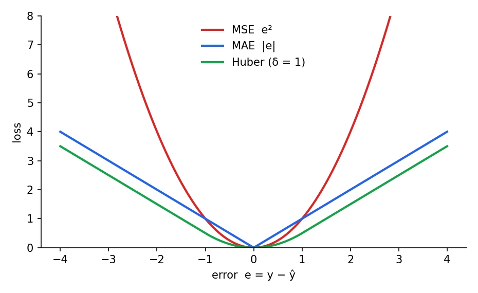
Look at the numbers. There are four small misses (all under 1) and one outlier of 8. The mean MSE is 12.97, and 99 percent of it comes from that single outlier. MAE gives 1.96, and Huber sits in between at 1.59. If that outlier is a data-entry error, MSE would drag your model towards it. If it is a real and important event, MSE's loudness is what you want. The loss is how you tell the model what to care about.
Losses for classification
Binary cross-entropy (log loss)
When a model outputs a probability that an example belongs to class 1, we need a loss that is small when the model is confidently right and huge when it is confidently wrong. Cross-entropy does exactly that.
is the true label (0 or 1) and is the predicted probability of class 1. If the loss is , and if it is . Only one of the two terms is ever active.
import numpy as np
import torch
import torch.nn.functional as F
import matplotlib.pyplot as plt

# Binary cross-entropy when the true label is 1: loss = -log(p)
for p in [0.99, 0.9, 0.5, 0.1, 0.01]:
    print(f"model says P(class 1) = {p:<5}  ->  loss {-np.log(p):.3f}")

# Softmax turns raw scores (logits) into probabilities that sum to 1
logits = torch.tensor([[2.0, 1.0, 0.1]])
probs = torch.softmax(logits, dim=1)
print("\nlogits :", logits.numpy().round(1)[0])
print("softmax:", probs.numpy().round(3)[0], " sum =", round(probs.sum().item(), 3))

true_class = torch.tensor([0])
by_hand = -torch.log(probs[0, 0])
by_torch = F.cross_entropy(logits, true_class)
print(f"cross-entropy by hand {by_hand.item():.4f}  | PyTorch {by_torch.item():.4f}")

p = np.linspace(0.01, 1, 200)
fig, ax = plt.subplots(figsize=(5.6, 3.5))
ax.plot(p, -np.log(p), lw=2.2, color="#7C3AED")
ax.set_xlabel("probability given to the correct class"); ax.set_ylabel("loss")
ax.spines[["top", "right"]].set_visible(False)
fig.tight_layout()model says P(class 1) = 0.99 -> loss 0.010
model says P(class 1) = 0.9 -> loss 0.105
model says P(class 1) = 0.5 -> loss 0.693
model says P(class 1) = 0.1 -> loss 2.303
model says P(class 1) = 0.01 -> loss 4.605
logits : [2. 1. 0.1]
softmax: [0.659 0.242 0.099] sum = 1.0
cross-entropy by hand 0.4170 | PyTorch 0.4170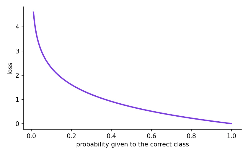
Read the first block as a story. The true label is 1. When the model says 0.99, the loss is a tiny 0.010. At 0.5 (a shrug) it is 0.693. At 0.1, the model is confidently wrong and the loss is 2.303. At 0.01 it is 4.605. The loss grows without limit as the model gets more confidently wrong. That steep punishment is the point: it is a very strong learning signal exactly when the model is most mistaken.
Categorical cross-entropy and softmax
For more than two classes, the output layer produces one raw score per class (called logits), and the softmax function turns them into probabilities that sum to 1:
is the score for class and is the number of classes. Exponentials make every value positive, and dividing by the total makes them add up to 1. The biggest score gets the biggest share. Because they compete for one total, softmax only makes sense when exactly one class is right.
The loss is then the negative log of the probability given to the correct class:
is 1 for the true class and 0 for the others (one-hot), so every term vanishes except the one for the true class. The output above confirms it: by hand the loss for the logits [2.0, 1.0, 0.1] with true class 0 is 0.4170, and PyTorch gives the same.
Cross-entropy comes from information theory, founded by Claude Shannon in his 1948 paper "A Mathematical Theory of Communication". Minimising it means the model is as little surprised by the true answers as it can be.Shannon, 1948
Hinge loss
One more you will meet in Session 14: hinge loss, the loss that support vector machines use. It does not care about probabilities. It only asks that the correct class wins by at least a safe margin, and ignores examples that are already far on the right side.
Which loss is the usual choice for a multi-class classifier such as a digit recogniser (0 to 9)?
Activation functions: why networks need them
Here is the problem. A neuron computes a weighted sum, . That is a straight-line (linear) operation. Stack ten layers of straight-line operations and you still have a straight line, no matter how deep you go. You can check it in four lines of code:
import numpy as np

rng = np.random.default_rng(0)
x = rng.normal(size=(5, 4))                 # 5 examples, 4 features
W1 = rng.normal(size=(4, 8))                # layer 1: 4 -> 8
W2 = rng.normal(size=(8, 3))                # layer 2: 8 -> 3

two_layers = (x @ W1) @ W2                  # stack two linear layers
one_layer = x @ (W1 @ W2)                   # ...it is the same as ONE layer with W = W1 @ W2
print("two linear layers == one linear layer:", np.allclose(two_layers, one_layer))

with_relu = np.maximum(0, x @ W1) @ W2      # put a ReLU in between
print("with a ReLU in between == one linear layer:", np.allclose(with_relu, one_layer))two linear layers == one linear layer: True
with a ReLU in between == one linear layer: FalseTwo linear layers are exactly the same as one layer with a combined weight matrix. Put a ReLU between them and the equality breaks. That small bend is what lets a network draw curved boundaries and learn complicated patterns.
First the weighted sum , then the activation function ("phi") bends it. The result is called the neuron's activation, and it is what gets passed to the next layer.
The four you must know
Sigmoid squeezes any number into the range 0 to 1. It is the natural choice for the output of a binary classifier, since the result reads as a probability.
Output in (0, 1). Its slope is at most 0.25, which will matter a lot in Session 8.
Tanh is a stretched and shifted sigmoid with output between -1 and 1, centred on zero, which often makes optimisation easier than with sigmoid.
Output in (-1, 1) and zero-centred. Its slope is at most 1, but like sigmoid it flattens out for large positive or negative inputs.
ReLU (Rectified Linear Unit) is the default for hidden layers. It is almost embarrassingly simple: pass positive numbers through, turn negative numbers into zero.
Cheap to compute, and its slope is exactly 1 for positive inputs, so gradients flow through it without shrinking. The weakness: a neuron whose input is always negative outputs zero forever and stops learning, the "dying ReLU" problem. Leaky ReLU keeps a small slope (such as 0.1) on the negative side to avoid it.
Softmax, which you met above, is for the output layer of multi-class problems.
import numpy as np
import matplotlib.pyplot as plt

x = np.linspace(-6, 6, 400)
sigmoid = 1 / (1 + np.exp(-x))
tanh = np.tanh(x)
relu = np.maximum(0, x)
leaky = np.where(x > 0, x, 0.1 * x)

fig, ax = plt.subplots(1, 2, figsize=(10.5, 3.8))
for y, name, c in [(sigmoid, "sigmoid", "#2563EB"), (tanh, "tanh", "#7C3AED"), (relu, "ReLU", "#16A34A"), (leaky, "Leaky ReLU", "#F59E0B")]:
    ax[0].plot(x, y, lw=2, color=c, label=name)
ax[0].set_ylim(-1.5, 3); ax[0].set_title("The functions"); ax[0].legend(frameon=False)

ax[1].plot(x, sigmoid * (1 - sigmoid), lw=2, color="#2563EB", label="sigmoid'")
ax[1].plot(x, 1 - tanh ** 2, lw=2, color="#7C3AED", label="tanh'")
ax[1].plot(x, (x > 0).astype(float), lw=2, color="#16A34A", label="ReLU'")
ax[1].set_title("Their slopes (what backprop multiplies by)"); ax[1].legend(frameon=False)
for a in ax:
    a.axhline(0, color="#9CA3AF", lw=.8); a.axvline(0, color="#9CA3AF", lw=.8); a.spines[["top", "right"]].set_visible(False)
fig.tight_layout()

z = np.array([-2.0, 0.0, 3.0])
print("z          ", z)
print("sigmoid    ", (1 / (1 + np.exp(-z))).round(3))
print("tanh       ", np.tanh(z).round(3))
print("ReLU       ", np.maximum(0, z))
print("max slope of sigmoid:", (sigmoid * (1 - sigmoid)).max().round(3), "| of tanh:", (1 - tanh ** 2).max().round(3))z [-2. 0. 3.]
sigmoid [0.119 0.5 0.953]
tanh [-0.964 0. 0.995]
ReLU [0. 0. 3.]
max slope of sigmoid: 0.25 | of tanh: 1.0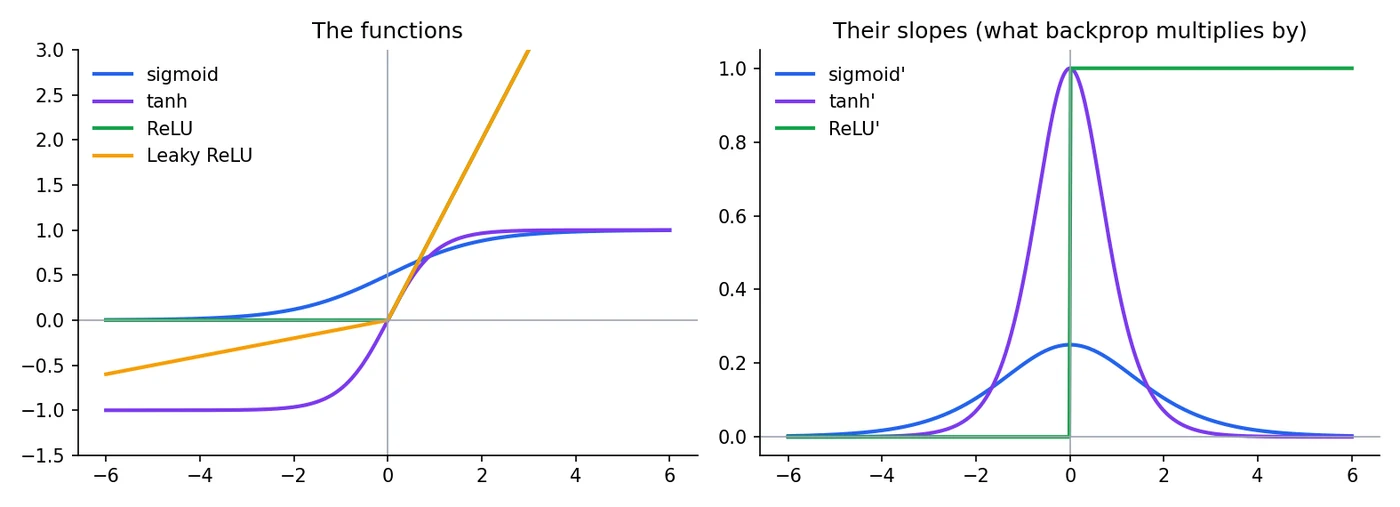
The left panel is the shapes. The right panel is the part that matters for training: the slope. Sigmoid's slope peaks at 0.25 and falls to nearly zero on both sides, so a neuron pushed into the flat region barely learns. ReLU's slope is a clean 1 for positive input. The printed values at the bottom show each function at -2, 0 and 3.
The 2012 AlexNet paper, which kicked off the modern deep-learning boom in image recognition, used ReLU instead of tanh and reported that its networks trained several times faster as a result.Krizhevsky, Sutskever and Hinton, 2012
Which one, where
| Function | Output range | Where it goes | Main strength | Main weakness |
|---|---|---|---|---|
| Sigmoid | (0, 1) | Output of a binary classifier | Reads as a probability | Vanishing gradients, not zero-centred |
| Tanh | (-1, 1) | Hidden layers of small networks | Zero-centred | Vanishing gradients |
| ReLU | [0, infinity) | Hidden layers (the default) | Fast, healthy gradients | "Dying" neurons |
| Softmax | (0, 1), sums to 1 | Output of a multi-class classifier | Gives a probability split | Needs mutually exclusive classes |
A rule of thumb that covers most cases: ReLU in the hidden layers, sigmoid for binary output, softmax for multi-class output, nothing for regression output (let it be any number).
import torch
import torch.nn as nn

x = torch.tensor([-2.0, 0.0, 3.0])
print(torch.sigmoid(x), torch.tanh(x), torch.relu(x))
print(torch.softmax(torch.tensor([2.0, 1.0, 0.1]), dim=0))      # probabilities, sum to 1

mse   = nn.MSELoss()              # regression (L2)
mae   = nn.L1Loss()               # regression (L1)
huber = nn.HuberLoss()            # regression, robust to outliers
bce   = nn.BCEWithLogitsLoss()    # binary classification
ce    = nn.CrossEntropyLoss()     # multi-class classification
print(ce(torch.tensor([[2.0, 0.5, 0.1]]), torch.tensor([0]))) # logits vs true class indexnn.CrossEntropyLoss and nn.BCEWithLogitsLoss take raw logits and apply softmax or sigmoid inside. If you add a softmax or sigmoid layer yourself before them, you apply it twice and training quietly gets worse.
What would happen if every layer of a deep network used no activation function at all?
Try it yourself
- In
losses.py, change the outlier from 8.0 to 2.0. Does the outlier still make up almost all of the MSE? - Plot the softplus function, , next to ReLU. It is a smooth version of ReLU. Why might smoothness not be worth the extra cost?
- Compute the softmax of
[1000, 1001, 1002]with the plain formula. What breaks? (Hint: overflow. Real libraries subtract the largest score first.) - Use
nn.BCEWithLogitsLosson a prediction of 0.5 logits and a true label of 1. Check it against-log(sigmoid(0.5)).
What comes next
We now have a loss that says how wrong the model is. The next question is how to reduce it. Session 7 is about the algorithm that walks downhill on the loss: gradient descent, its variants and the optimisers like Adam that are built on it.
Frequently asked questions
What is the difference between a loss function and a cost function?
A loss function measures the error on a single training example. A cost function averages the loss over the whole dataset or a batch, and is the number that gradient descent minimises. In everyday use people often say loss for both.
Why can't I use MSE for classification?
You can, but it works poorly. MSE gives weak gradients when the model is confidently wrong, and it does not treat outputs as probabilities. Cross-entropy punishes confident mistakes heavily, which gives a stronger learning signal and better results.
Why is ReLU the default activation in hidden layers?
It is cheap to compute and its slope is exactly 1 for positive inputs, so gradients do not shrink as they pass through many layers. That makes deep networks much easier to train than with sigmoid or tanh.
What is the dying ReLU problem?
If a neuron's input is negative for every training example, ReLU outputs zero and its gradient is zero, so the neuron never updates again. Leaky ReLU, a lower learning rate and good initialisation reduce the problem.
When should I use sigmoid and when softmax?
Use sigmoid for a binary output, one probability for yes or no, and also for multi-label problems where several labels can be true at once. Use softmax when exactly one class out of several is correct.