
A model that scores "95 percent" can still be useless. A model with an R² of 0.45 can still be valuable. Numbers do not mean anything until you know which number, measured on which data, against which baseline. This session is about choosing the right yardstick, because the wrong one will happily tell you your model is great while it quietly fails.
You already met R² in Session 2 and compared models in Session 3. Now we do it properly, first for models that predict numbers (regression) and then for models that predict categories (classification).
Why the metric matters
You choose a metric to match what a mistake costs you. Predicting a house price Rs. 200,000 too high is a different kind of problem from telling a patient a tumour is benign when it is not. One metric cannot speak for both. Always split the question in two: what kind of output do I have, and which mistakes hurt most.
| Task | Typical metrics |
|---|---|
| Regression (a number) | MAE, MSE, RMSE, R² |
| Classification (a category) | Confusion matrix, accuracy, precision, recall, F1 |
Remember too that every metric here should be computed on held-out data (the test set from Session 1), never on the data the model trained on.
Regression metrics
MAE: the average miss
Mean absolute error takes each prediction error, drops the sign and averages. It is in the same units as the target, so it is the easiest metric to explain to a non-technical person: "on average we are off by about 43 points."
is the actual value, the prediction and the number of rows. Every error counts in proportion to its size, so one huge outlier does not dominate the score.
MSE and RMSE: punishing the big misses
Mean squared error squares each error before averaging. Squaring makes large errors count far more, and it also makes the formula smooth, which is why MSE is the usual loss function for training (you used it in Session 1). The catch is its units: squared units, such as "squared marks", which are hard to picture. Taking the square root gives RMSE, back in the original units.
Use MSE or RMSE when large errors are especially costly. RMSE is always at least as big as MAE, and the more it exceeds MAE, the more your errors are dominated by a few big ones.
Here is that last remark in numbers. Ten predictions, small steady mistakes, and then the same predictions with one wild miss:
import numpy as np
from sklearn.metrics import mean_absolute_error, mean_squared_error

actual = np.array([100, 102, 98, 101, 99, 100, 103, 97, 100, 101])
good   = actual + np.array([2, -1, 1, -2, 1, 0, -1, 2, -1, 1])       # small, steady mistakes
one_bad = good.copy(); one_bad[3] = 160                              # same, but one wild miss

for name, pred in [("steady small errors", good), ("same + one wild miss", one_bad)]:
    mae = mean_absolute_error(actual, pred)
    rmse = np.sqrt(mean_squared_error(actual, pred))
print(f"{name:22s} MAE {mae:5.2f} RMSE {rmse:5.2f}")steady small errors MAE 1.20 RMSE 1.34
same + one wild miss MAE 6.90 RMSE 18.69MAE rises from 1.2 to 6.9. RMSE leaps from 1.3 to 18.7. Same ten predictions, one mistake. If a rare disaster is what you fear, RMSE will shout about it. If you want a fair "typical error", MAE is steadier.
R²: compared with just guessing the average
MAE and RMSE answer "how big are the errors?". R² answers a different question: "how much better is this model than a lazy one that always predicts the average?"
is the average of the actual values. The top is the model's error, the bottom is the error of always guessing . A score of 1 is perfect, 0 means no better than the average, and below 0 means the model is worse than the average. R² has no units, but it does not tell you how large the errors are in practice.
Time to score four models on the diabetes data, including the lazy "always predict the mean" baseline, which every real model must beat.
import numpy as np
from sklearn.datasets import load_diabetes
from sklearn.dummy import DummyRegressor
from sklearn.linear_model import LinearRegression, Ridge, Lasso
from sklearn.metrics import mean_absolute_error, mean_squared_error, r2_score
from sklearn.model_selection import train_test_split
from sklearn.pipeline import make_pipeline
from sklearn.preprocessing import StandardScaler

X, y = load_diabetes(return_X_y=True)
X_tr, X_te, y_tr, y_te = train_test_split(X, y, test_size=0.2, random_state=42)

models = {
    "Always predict the mean": DummyRegressor(strategy="mean"),
    "Linear regression": LinearRegression(),
    "Ridge (alpha=10)": Ridge(alpha=10),
    "Lasso (alpha=2)": Lasso(alpha=2),
}
print(f"{'model':26s} {'MAE':>6s} {'MSE':>8s} {'RMSE':>6s} {'R²':>7s}")
for name, est in models.items():
    pred = make_pipeline(StandardScaler(), est).fit(X_tr, y_tr).predict(X_te)
    mae = mean_absolute_error(y_te, pred); mse = mean_squared_error(y_te, pred)
print(f"{name:26s} {mae:6.1f} {mse:8.1f} {np.sqrt(mse):6.1f} {r2_score(y_te, pred):7.3f}")model MAE MSE RMSE R²
Always predict the mean 64.0 5361.5 73.2 -0.012
Linear regression 42.8 2900.2 53.9 0.453
Ridge (alpha=10) 42.9 2875.8 53.6 0.457
Lasso (alpha=2) 42.8 2798.9 52.9 0.472Three lessons are packed in there.
- The baseline's R² is -0.012, slightly below zero. That is how a negative R² happens in real life: guessing the training average is a little off for the test rows.
- Moving from baseline to linear regression cuts MAE from 64.0 to 42.8, and lifts R² from about 0 to 0.45. Now we know how much the features actually buy us.
- The three real models are separated by tiny margins. Lasso has the best RMSE and R², but the gap is small enough that a different split could reorder them. Do not crown a winner on a 0.01 difference from one test set.
The Netflix Prize (2006 to 2009) offered $1 million to anyone who could cut the error of Netflix's movie-rating predictions, measured by RMSE, by 10 percent. A team called BellKor's Pragmatic Chaos won it.Netflix Prize, 2009
A model gets R² = -0.4 on the test set. What does that tell you?
Classification metrics
When the output is a category, an average error makes no sense. Instead, we count how often each kind of answer was right or wrong. The starting point is the confusion matrix.
For a yes/no question, call "yes" the positive class (in the next example, a tumour being malignant). Every prediction lands in one of four boxes:
| Predicted positive | Predicted negative | |
|---|---|---|
| Actually positive | TP (true positive): correctly flagged | FN (false negative): a real case we missed |
| Actually negative | FP (false positive): a false alarm | TN (true negative): correctly cleared |
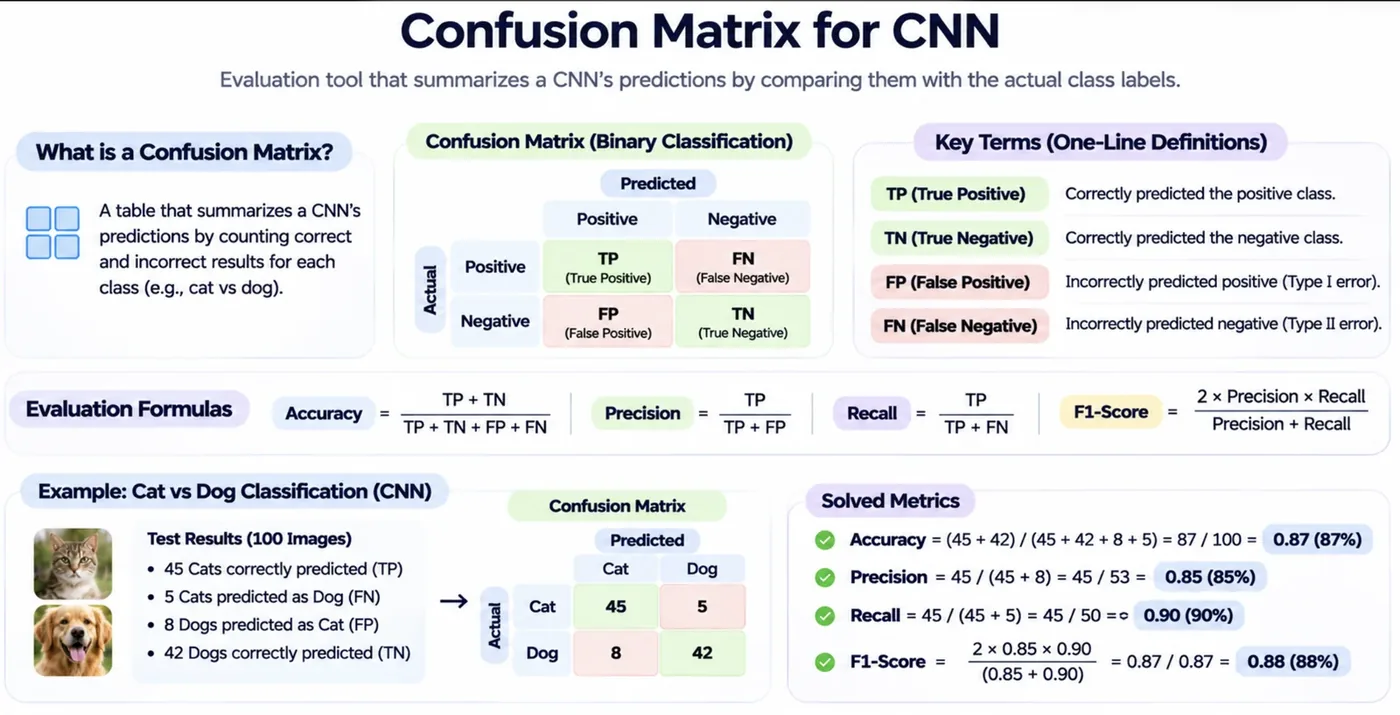
From those four counts come all the classification metrics. Here they are, each with the question it answers.
"Out of everything, how often was the model right?" Simple, and misleading when one class is rare (see the trap below).
"When the model says positive, how often is it right?" High precision means few false alarms. It matters when a false alarm is expensive, like marking a good email as spam.
"Of all the real positives, how many did the model find?" High recall means few misses. It matters when a miss is expensive, like overlooking a disease.
The harmonic mean of precision and recall. It is dragged down by whichever of the two is weaker, so you cannot hide a bad recall behind a great precision. Use it when classes are imbalanced and you care about both kinds of mistake.
A real example
We now train a simple classifier (logistic regression, Session 5 introduces it properly) on the Wisconsin breast-cancer dataset that ships with scikit-learn: 569 tumour samples, each described by 30 measurements. We mark "malignant" as the positive class, because it is the one we cannot afford to miss.
import matplotlib.pyplot as plt
from sklearn.datasets import load_breast_cancer
from sklearn.linear_model import LogisticRegression
from sklearn.metrics import ConfusionMatrixDisplay, classification_report, confusion_matrix
from sklearn.model_selection import train_test_split
from sklearn.pipeline import make_pipeline
from sklearn.preprocessing import StandardScaler

data = load_breast_cancer()
y = (data.target == 0).astype(int)        # make 1 = malignant, the thing we want to catch
X_tr, X_te, y_tr, y_te = train_test_split(data.data, y, test_size=0.25, random_state=42, stratify=y)

clf = make_pipeline(StandardScaler(), LogisticRegression(max_iter=1000)).fit(X_tr, y_tr)
pred = clf.predict(X_te)

cm = confusion_matrix(y_te, pred)
tn, fp, fn, tp = cm.ravel()
print("confusion matrix (rows = actual, columns = predicted):")
print(cm)
print(f"TP={tp}  FN={fn}  FP={fp}  TN={tn}\n")
print(classification_report(y_te, pred, target_names=["benign", "malignant"], digits=3))

fig, ax = plt.subplots(figsize=(4.6, 3.8))
ConfusionMatrixDisplay(cm, display_labels=["benign", "malignant"]).plot(ax=ax, cmap="Blues", colorbar=False)
ax.set_title("Breast-cancer classifier")
fig.tight_layout()confusion matrix (rows = actual, columns = predicted):
[[89 1]
[ 4 49]]
TP=49 FN=4 FP=1 TN=89
precision recall f1-score support
benign 0.957 0.989 0.973 90
malignant 0.980 0.925 0.951 53
accuracy 0.965 143
macro avg 0.968 0.957 0.962 143
weighted avg 0.966 0.965 0.965 143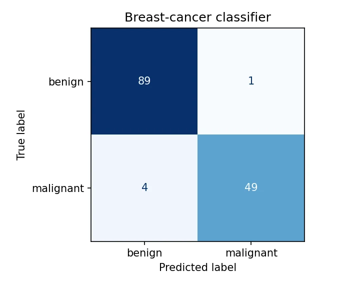
Walk through the matrix. Of the 53 truly malignant tumours, the model caught 49 (TP) and missed 4 (FN). Of the 90 benign ones, it cleared 89 (TN) and raised 1 false alarm (FP). Now each metric is just arithmetic on those counts:
- Accuracy = (49 + 89) / 143 = 0.965.
- Precision for malignant = 49 / (49 + 1) = 0.980.
- Recall for malignant = 49 / (49 + 4) = 0.925.
Notice what accuracy hides. The 4 missed tumours are the real failure in a medical setting, and recall (0.925) shows it more clearly than a 96.5 percent headline. The report's other columns: support is the number of real samples in each class, the macro average is the plain average across classes (each class counts the same), and the weighted average weighs each class by its support.
The accuracy trap
Suppose 5 percent of emails are spam, and someone gives you a "model" that always answers "not spam".
import numpy as np
from sklearn.metrics import accuracy_score, precision_score, recall_score, f1_score

# 1000 emails, only 50 are spam (5%)
y_true = np.array([1] * 50 + [0] * 950)
y_lazy = np.zeros(1000, dtype=int)                   # a "model" that always says: not spam

print("accuracy :", accuracy_score(y_true, y_lazy))
print("recall   :", recall_score(y_true, y_lazy))
print("precision:", precision_score(y_true, y_lazy, zero_division=0))
print("F1 :", f1_score(y_true, y_lazy, zero_division=0))accuracy : 0.95
recall : 0.0
precision: 0.0
F1 : 0.095 percent accuracy, and yet it catches zero spam: recall, precision and F1 are all 0. Whenever one class is much rarer than the other (fraud, disease, defects), accuracy is almost meaningless. Look at precision, recall and F1 for the rare class instead.
A fraud model must catch as many fraudulent transactions as possible, even if it flags some honest ones by mistake. Which metric should you push up first?
Precision and recall pull against each other
Most classifiers output a probability, and a threshold turns it into a yes/no answer. Lower the threshold and the model says "positive" more often. You catch more real cases (recall rises) but raise more false alarms (precision falls). Raise it and the opposite happens.
from sklearn.datasets import load_breast_cancer
from sklearn.linear_model import LogisticRegression
from sklearn.metrics import precision_score, recall_score
from sklearn.model_selection import train_test_split
from sklearn.pipeline import make_pipeline
from sklearn.preprocessing import StandardScaler

data = load_breast_cancer()
y = (data.target == 0).astype(int)
X_tr, X_te, y_tr, y_te = train_test_split(data.data, y, test_size=0.25, random_state=42, stratify=y)
clf = make_pipeline(StandardScaler(), LogisticRegression(max_iter=1000)).fit(X_tr, y_tr)
p = clf.predict_proba(X_te)[:, 1]                    # the model's probability of "malignant"

print("threshold  precision  recall")
for t in [0.1, 0.3, 0.5, 0.7, 0.9]:
    pred = (p >= t).astype(int)
print(f" {t:.1f} {precision_score(y_te, pred):.3f} {recall_score(y_te, pred):.3f}")threshold precision recall
0.1 0.897 0.981
0.3 0.981 0.962
0.5 0.980 0.925
0.7 1.000 0.906
0.9 1.000 0.811At a threshold of 0.1 the model finds 98.1 percent of the malignant tumours but only 89.7 percent of its alarms are correct. At 0.9 every alarm is correct (precision 1.000) but it now misses almost 19 percent of real cases. The default threshold of 0.5 is not sacred. For a cancer screen you would probably choose a low threshold and accept extra follow-up checks; for an automatic account ban you would choose a high one.
The breast-cancer dataset used here comes from Wisconsin and describes 569 tumour samples with 30 measurements taken from digitised images of cell nuclei.Wolberg, Street and Mangasarian, UCI Machine Learning Repository
Which metric, when?
| Your situation | Lean on |
|---|---|
| Numbers, errors in plain units wanted | MAE |
| Numbers, big misses are costly | RMSE or MSE |
| Numbers, want a "how much better than average" score | R² (plus an error metric) |
| Classes, balanced, all mistakes cost the same | Accuracy |
| Classes, false alarms are costly | Precision |
| Classes, misses are costly | Recall |
| Classes, imbalanced, want one number | F1 |
from sklearn.metrics import (mean_absolute_error, mean_squared_error, r2_score,
                             confusion_matrix, classification_report)

# regression
print(mean_absolute_error(y_test, y_pred_reg),
      mean_squared_error(y_test, y_pred_reg),
      r2_score(y_test, y_pred_reg))

# classification
print(confusion_matrix(y_test, y_pred_clf))
print(classification_report(y_test, y_pred_clf))
Try it yourself
- In
regression_metrics.py, changerandom_state=42to 7 and 99. Does the ranking of the models stay the same? What does that say about trusting a single split? - Edit
outlier_effect.pyso the wild miss is 130 instead of 160. How do MAE and RMSE move? - In
threshold.py, find a threshold where recall is at least 0.97. What precision do you pay for it? - Build a "model" that always predicts the majority class on the cancer data. What accuracy does it get, and what is its recall for malignant?
What comes next
Now you can score a model honestly. But so far every setting (alpha, the test size, the threshold) was chosen by hand. Session 5 is about those settings, the hyperparameters, and how to tune them systematically without cheating on the test set.
Frequently asked questions
What is the difference between MAE, MSE and RMSE?
MAE is the average absolute error, in the same units as the target. MSE averages the squared errors, so large mistakes count much more, but its units are squared. RMSE is the square root of MSE, which brings it back to the original units. RMSE is always at least as large as MAE, and a big gap between them means a few large errors dominate.
Can R-squared be negative?
Yes, on test data. R² compares your model with a baseline that always predicts the mean. If your model's errors are bigger than that baseline's, R² drops below zero. On training data for ordinary least squares it cannot be negative.
What is the difference between precision and recall?
Precision asks "of the items the model labelled positive, how many really were?" and punishes false alarms. Recall asks "of the items that really were positive, how many did the model find?" and punishes misses. Which to prioritise depends on which mistake costs more.
Why is accuracy a bad metric for imbalanced data?
Because a model can score high by always predicting the common class. If 95 percent of emails are not spam, always answering "not spam" is 95 percent accurate while catching no spam at all. Use precision, recall and F1 for the rare class instead.
What is a good F1 score?
There is no universal cut-off. Compare against a simple baseline and against what your use case needs. F1 of 0.95 on a balanced, easy task may be ordinary, while 0.6 on a hard imbalanced task may be a real achievement.