LSTM Explained: The Cell State and the Forget, Input and Output Gates, Step by Step

Last session ended with a measurement: a plain RNN's learning signal fades by thirteen orders of magnitude across 60 steps, so it forgets the start of a long sequence. The Long Short-Term Memory (LSTM) network, published by Sepp Hochreiter and Jürgen Schmidhuber in 1997, was designed to fix exactly that. It dominated speech, translation and time-series work for almost two decades.

An LSTM is not complicated once you see it as a conveyor belt with three switches. This session computes one step by hand, shows why the design lets information and gradients travel far, and then tests it honestly, including a result that did not go the way the textbook story suggests. You need the RNN from Session 18 and the vanishing-gradient idea from Session 8.

The idea: a protected memory line

A plain RNN has one memory, the hidden state, and rewrites it completely at every step. Every rewrite squashes the old content through a $\tanh$ and a weight matrix, which is how information gets lost.

The LSTM keeps two pieces of state:

• the cell state $c_t$: the long-term memory, a "conveyor belt" that runs straight through time with only small, controlled edits;
• the hidden state $h_t$: the short-term output that is shown to the rest of the network.

And it uses three gates, each a sigmoid that outputs numbers between 0 (block) and 1 (let through), to control what happens to the belt:

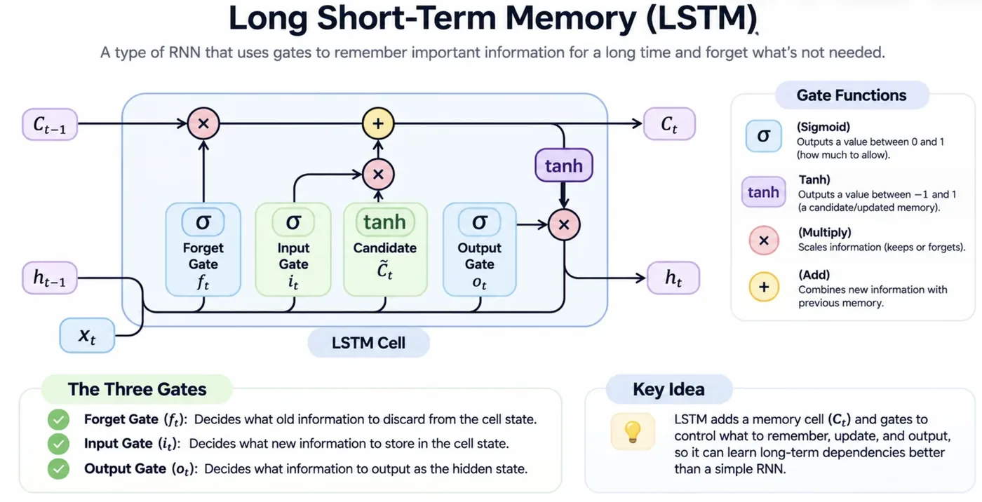
• Forget gate $f_t$: how much of the old memory to keep (0 = forget everything, 1 = keep it all).
• Input gate $i_t$: how much of the new candidate information to write onto the belt.
• Output gate $o_t$: how much of the memory to reveal as the new hidden state.

The equations

At each step the cell sees the current input $x_t$ and the previous hidden state $h_{t-1}$, joined together. Four small layers use them:

Then the gates act on the memory:

Let us run exactly one step with real numbers and then check it against PyTorch:

import numpy as np
import torch
import torch.nn as nn

sigmoid = lambda z: 1 / (1 + np.exp(-z))
rng = np.random.default_rng(0)
n_in, n_hid = 3, 4

# one LSTM step: four sets of weights (forget, input, candidate, output) acting on [x_t, h_{t-1}]
W = {g: rng.normal(size=(n_in + n_hid, n_hid)) * 0.6 for g in "figo"}
b = {g: np.zeros(n_hid) for g in "figo"}

x_t = rng.normal(size=n_in)
h_prev = rng.normal(size=n_hid) * 0.5
c_prev = rng.normal(size=n_hid)                          # the long-term memory carried in
z = np.concatenate([x_t, h_prev])

f = sigmoid(z @ W["f"] + b["f"])                          # forget gate : how much of the old memory to keep (0..1)
i = sigmoid(z @ W["i"] + b["i"])                          # input gate  : how much of the new candidate to write (0..1)
g = np.tanh(z @ W["g"] + b["g"])                          # candidate   : the new information (-1..1)
o = sigmoid(z @ W["o"] + b["o"])                          # output gate : how much of the memory to expose (0..1)

c_t = f * c_prev + i * g                                  # update the conveyor belt
h_t = o * np.tanh(c_t)                                    # the short-term output

print("old memory c_prev :", c_prev.round(2))
print("forget gate f     :", f.round(2))
print("input gate  i     :", i.round(2))
print("new memory  c_t   :", c_t.round(2))
print("output gate o     :", o.round(2))
print("hidden state h_t  :", h_t.round(2))

# check against PyTorch's LSTMCell (its gate order is input, forget, candidate, output)
cell = nn.LSTMCell(n_in, n_hid)
with torch.no_grad():
    cell.weight_ih.copy_(torch.tensor(np.concatenate([W[k][:n_in].T for k in "ifgo"])))
    cell.weight_hh.copy_(torch.tensor(np.concatenate([W[k][n_in:].T for k in "ifgo"])))
    cell.bias_ih.zero_(); cell.bias_hh.zero_()
    h_torch, c_torch = cell(torch.tensor(x_t, dtype=torch.float32)[None], (torch.tensor(h_prev, dtype=torch.float32)[None], torch.tensor(c_prev, dtype=torch.float32)[None]))
print("\nmatches torch.nn.LSTMCell:", np.allclose(h_torch[0].numpy(), h_t, atol=1e-5) and np.allclose(c_torch[0].numpy(), c_t, atol=1e-5))

old memory c_prev : [1.16 0.79 0.84 0.08]
forget gate f     : [0.53 0.44 0.5  0.64]
input gate  i     : [0.63 0.49 0.61 0.76]
new memory  c_t   : [0.78 0.35 0.99 0.02]
output gate o     : [0.4  0.56 0.49 0.64]
hidden state h_t  : [0.26 0.19 0.37 0.01]

matches torch.nn.LSTMCell: True

Read it as a story for each of the four memory slots. Slot 1 had an old memory of 1.16. The forget gate was 0.53, so about half of it was kept, the input gate was 0.63 and let in part of the new candidate, and the new memory became 0.78. The output gate of 0.4 then decided that only a fraction of that is shown as the hidden state, 0.26. Each slot makes its own decisions. The last line confirms PyTorch's LSTMCell gives the same answer.

Why this helps: a highway for gradients

Look at how the cell state changes from one step to the next: $c_t = f_t \odot c_{t-1} + \dots$. If you ask how $c_t$ depends on $c_{t-1}$, the answer is simply the forget gate:

Let's measure that instead of just claiming it. We run three kinds of recurrent layer, untrained, over 100 steps and ask how much an input $k$ steps back still affects the final hidden state, averaged over ten random starts. For the LSTM we use a well-known trick, starting the forget gate's bias at 1 so it leans towards "remember".

import matplotlib.pyplot as plt
import numpy as np
import torch
import torch.nn as nn

T, hidden, runs = 100, 32, 10

def influence(kind, forget_bias=None):
    """How much does the input k steps ago still change the final hidden state? (averaged over random starts)"""
    total = np.zeros(T)
    for seed in range(runs):
        torch.manual_seed(seed)
        layer = {"RNN": nn.RNN, "GRU": nn.GRU, "LSTM": nn.LSTM}[kind](1, hidden, batch_first=True)
        if forget_bias is not None:
            for name, p in layer.named_parameters():
                if "bias_ih" in name: p.data[hidden:2 * hidden] = forget_bias        # the forget-gate slice
        x = torch.randn(1, T, 1, requires_grad=True)
        out, _ = layer(x)
        out[0, -1].norm().backward()
        total += x.grad[0, :, 0].abs().numpy()
    return total / runs

curves = {"RNN": influence("RNN"), "GRU": influence("GRU"), "LSTM (forget bias 1)": influence("LSTM", 1.0)}
for name, c in curves.items():
    print(f"{name:22s} influence of the input 50 steps back: {c[T - 1 - 50]:.1e}   99 steps back: {c[0]:.1e}")

fig, ax = plt.subplots(figsize=(6.6, 3.8))
for (name, c), col in zip(curves.items(), ["#DC2626", "#F59E0B", "#16A34A"]):
    ax.semilogy(range(T - 1, -1, -1), c + 1e-30, lw=2, color=col, label=name)
ax.set_xlabel("how many steps back the input was"); ax.set_ylabel("influence on the final state (log)")
ax.legend(frameon=False); ax.spines[["top", "right"]].set_visible(False)
fig.tight_layout()

RNN                    influence of the input 50 steps back: 2.6e-12   99 steps back: 2.1e-21
GRU                    influence of the input 50 steps back: 8.2e-12   99 steps back: 1.6e-20
LSTM (forget bias 1)   influence of the input 50 steps back: 8.7e-06   99 steps back: 9.8e-09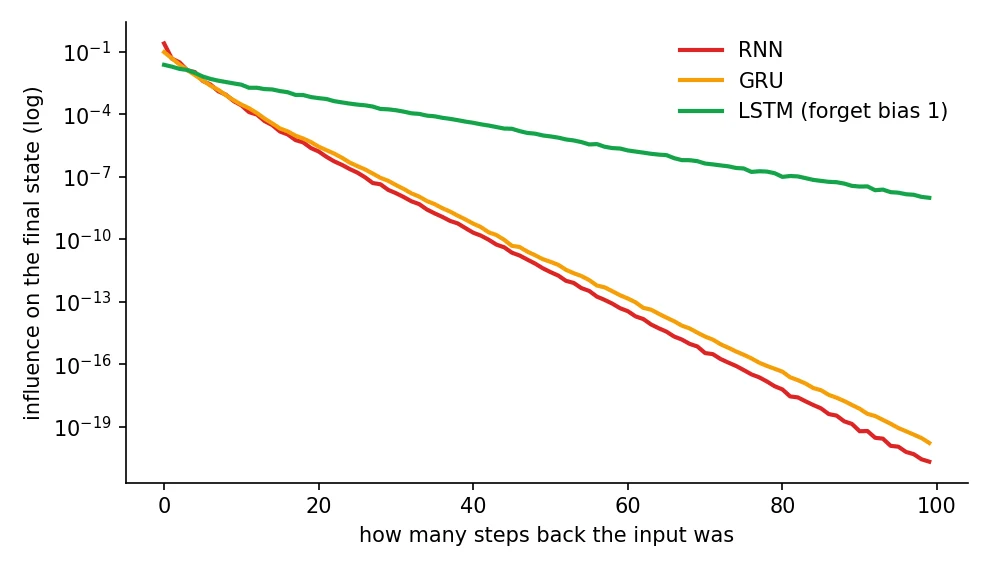

At 50 steps back, the plain RNN's influence is $2.6\times10^{-12}$ and the LSTM's is $8.7\times10^{-6}$, about three million times larger. At 99 steps back, $2.1\times10^{-21}$ against $9.8\times10^{-9}$. The LSTM's curve is far flatter. Notice that the GRU, at its default starting point, is not much better than the plain RNN (8.2e-12 at 50 steps). Gates only help once they are set to let things through, and a GRU's gates start around one half.

The cost: more parameters

Four sets of weights instead of one means four times the parameters of a plain RNN of the same size:

import torch.nn as nn

n_in, n_hid = 1, 64
count = lambda m: sum(p.numel() for p in m.parameters())
for name, layer, gates in [("RNN", nn.RNN, 1), ("GRU", nn.GRU, 3), ("LSTM", nn.LSTM, 4)]:
    formula = gates * (n_hid * (n_in + n_hid) + 2 * n_hid)      # PyTorch keeps two bias vectors per gate
    print(f"{name:5s} parameters: {count(layer(n_in, n_hid)):6,d}   formula {gates} x (h(x+h) + 2h) = {formula:,}")

RNN   parameters:  4,288   formula 1 x (h(x+h) + 2h) = 4,288
GRU   parameters: 12,864   formula 3 x (h(x+h) + 2h) = 12,864
LSTM  parameters: 17,152   formula 4 x (h(x+h) + 2h) = 17,152

With 64 hidden units and one input, the RNN has 4,288 parameters, the GRU 12,864 and the LSTM 17,152. The formula predicts all three exactly.

GRU: a lighter cousin

The Gated Recurrent Unit (GRU), introduced by Kyunghyun Cho and colleagues in 2014, simplifies the LSTM: it merges the cell and hidden state into one, and uses two gates (update and reset) instead of three. It has about three quarters of the LSTM's parameters, trains faster, and often performs about as well. Treat the choice between them as something to try, not to settle by theory.

Honest tests

Does it fix the memory test?

Last session's memory task was: label = sign of the first number, the rest is noise. A plain RNN fell to chance by 60 steps. Surely the LSTM fixes it? Try, with the same settings, for all three layers:

import torch
import torch.nn as nn

def make_batch(batch, T):
    x = torch.randn(batch, T, 1)                      # the label is the sign of the FIRST number, the rest is noise
    return x, (x[:, 0, 0] > 0).float()

class Net(nn.Module):
    def __init__(self, kind):
        super().__init__()
        self.rnn = {"RNN": nn.RNN, "GRU": nn.GRU, "LSTM": nn.LSTM}[kind](1, 32, batch_first=True)
        self.head = nn.Linear(32, 1)
    def forward(self, x):
        _, h = self.rnn(x)
        h = h[0] if isinstance(h, tuple) else h
        return self.head(h[-1]).squeeze(-1)

print("kind   length   accuracy, mean of 3 runs   (50% = guessing)")
for kind in ("RNN", "GRU", "LSTM"):
    for T in (10, 30):
        accs = []
        for seed in range(3):
            torch.manual_seed(seed)
            net = Net(kind); opt = torch.optim.Adam(net.parameters(), lr=0.01)
            for step in range(500):
                x, y = make_batch(64, T)
                loss = nn.functional.binary_cross_entropy_with_logits(net(x), y)
                opt.zero_grad(); loss.backward(); nn.utils.clip_grad_norm_(net.parameters(), 1.0); opt.step()
            x, y = make_batch(2000, T)
            accs.append(((net(x) > 0).float() == y).float().mean().item())
        print(f"{kind:5s}  {T:5d}     {sum(accs) / 3:.3f}")

kind   length   accuracy, mean of 3 runs   (50% = guessing)
RNN       10     0.990
RNN       30     0.715
GRU       10     0.998
GRU       30     0.496
LSTM      10     0.988
LSTM      30     0.504

Here is the honest result: it did not. At length 10 all three solve it (0.99 to 0.998). At length 30 the plain RNN still manages 0.715 on average, but the GRU and the LSTM stay at chance (about 0.50) after 500 steps of training. It is a real and well-known behaviour, not a bug. The gates are not magic: they have to be learned, and here the model has no cue telling it which of the 30 numbers is the one to keep. The network must discover "write the first input and then refuse every later one", which gives a flat, hard-to-find signal. Gated networks can solve such problems with much more training, a forget-gate bias, or a task that includes a marker, but not on a short budget.

The measurement above shows the gated cell can carry gradients far, while this test shows that using that ability still takes training. Both are true, and a textbook that shows only one of them is selling you something.

Forecasting a time series

Now a more practical comparison. The same made-up daily series as last session, windows of 30 days, and all three layers trained identically (three runs each), plus the "same as yesterday" baseline:

import numpy as np
import matplotlib.pyplot as plt
import torch
import torch.nn as nn

rng = np.random.default_rng(1)
t = np.arange(1500)
series = 25 + 10 * np.sin(2 * np.pi * t / 365) + 0.004 * t + rng.normal(0, 1.5, len(t))     # same made-up daily series as Session 18
series = (series - series.mean()) / series.std()

def make_windows(s, seq_len):
    X = np.array([s[i:i + seq_len] for i in range(len(s) - seq_len)])
    return X[..., None], s[seq_len:]

seq_len, split = 30, 1100
X, y = make_windows(series, seq_len)
X_tr, y_tr, X_te, y_te = [torch.tensor(a, dtype=torch.float32) for a in (X[:split], y[:split], X[split:], y[split:])]

class Forecaster(nn.Module):
    def __init__(self, kind):
        super().__init__()
        self.rnn = {"RNN": nn.RNN, "GRU": nn.GRU, "LSTM": nn.LSTM}[kind](1, 32, batch_first=True); self.head = nn.Linear(32, 1)
    def forward(self, x):
        _, h = self.rnn(x)
        h = h[0] if isinstance(h, tuple) else h                 # an LSTM also returns its cell state
        return self.head(h[-1]).squeeze(-1)

def fit(kind, seed):
    torch.manual_seed(seed); model = Forecaster(kind); opt = torch.optim.Adam(model.parameters(), lr=0.005)
    for epoch in range(40):
        perm = torch.randperm(len(X_tr))
        for i in range(0, len(perm), 64):
            b = perm[i:i + 64]
            loss = nn.functional.mse_loss(model(X_tr[b]), y_tr[b]); opt.zero_grad(); loss.backward(); opt.step()
    with torch.no_grad():
        return model, ((model(X_te) - y_te) ** 2).mean().item()

naive = ((X_te[:, -1, 0] - y_te) ** 2).mean().item()
print(f"{'model':28s} test MSE (mean of 3 runs)")
print(f"{'same as yesterday':28s} {naive:.3f}")
best = None
for kind in ("RNN", "GRU", "LSTM"):
    runs = [fit(kind, s) for s in range(3)]
    print(f"{kind:28s} {np.mean([r[1] for r in runs]):.3f}   (runs: {', '.join(f'{r[1]:.3f}' for r in runs)})")
    if kind == "LSTM": best = runs[0][0]

with torch.no_grad():
    pred = best(X_te)
fig, ax = plt.subplots(figsize=(8.2, 3.4))
ax.plot(y_te[:120].numpy(), color="#9CA3AF", lw=2, label="actual"); ax.plot(pred[:120].numpy(), color="#16A34A", lw=2, label="LSTM prediction")
ax.set_xlabel("day (test period)"); ax.set_ylabel("standardised value"); ax.legend(frameon=False); ax.spines[["top", "right"]].set_visible(False)
fig.tight_layout()

model                        test MSE (mean of 3 runs)
same as yesterday            0.104
RNN                          0.068   (runs: 0.071, 0.067, 0.066)
GRU                          0.061   (runs: 0.059, 0.064, 0.061)
LSTM                         0.063   (runs: 0.063, 0.062, 0.064)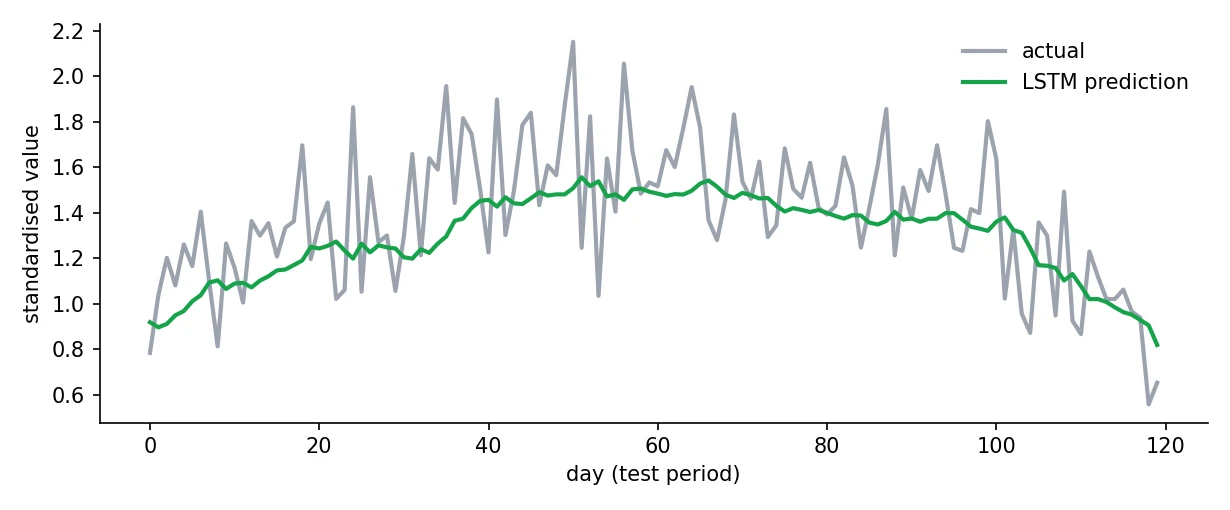

The naive baseline scores a squared error of 0.104. The plain RNN gets 0.068, the LSTM 0.063 and the GRU 0.061. All three beat the baseline clearly, and the gated layers are a bit better than the plain RNN, by around 7 to 10 percent. The gap between GRU and LSTM (0.002) is smaller than the run-to-run variation, so call those two equal. That is a fair summary of recurrent models in practice: gated cells help modestly on moderate sequences, and a lot more on long ones that the plain RNN cannot reach.

Using an LSTM

Sequence models want input shaped (samples, time steps, features). Turn a series into windows first:

import numpy as np
import torch.nn as nn

def make_windows(series, seq_len):
    X = np.array([series[i:i + seq_len] for i in range(len(series) - seq_len)])
    y = series[seq_len:]
    return X[..., None], y            # X shape: (samples, seq_len, 1)

lstm = nn.LSTM(input_size=1, hidden_size=64, num_layers=2, batch_first=True)
out, (h_n, c_n) = lstm(x)            # outputs for every step, plus the final hidden and cell states

A few habits that save hours: scale your series (Session 5), split by time and never shuffle across the split, always compare against the naive baseline, clip gradients (clip_grad_norm_) and give it enough epochs. Stock-price prediction deserves special caution: markets are close to random day to day, so a model that "predicts" a price curve often just copies yesterday's value.

Where LSTMs are used, and the next wall

LSTMs shine in speech recognition, handwriting recognition, time-series forecasting, anomaly detection in sensor streams, and in healthcare for tracking vital signs. For language tasks they have largely been replaced by Transformers, but they remain a strong, light choice for modest sequence problems, especially on small devices.

They carry two limits forward. First, an LSTM still reads one token at a time, so step 50 cannot start until step 49 is done, which wastes the parallel power of GPUs. Second, all the history is squeezed into one fixed-size memory vector, however long the sequence. A model that could look directly at any earlier word, and read the whole sequence in parallel, would remove both limits. That is the Transformer, and it is where Part V begins.

Part IV complete: what you can do now

You can explain how a CNN sees an image, run a YOLO detector, and describe how recurrent networks carry memory, why plain ones forget and how gates and a cell state help. You also know how to test such claims instead of trusting them: measure the gradient, compare against a baseline, repeat with several random starts.

Try it yourself

1. In gradient_flow.py, run the LSTM with forget_bias of 0 and then 3. How does the curve change?
2. In remember_first_gated.py, raise the training steps from 500 to 3,000 for the LSTM at length 30. Does it eventually learn?
3. In forecast_lstm.py, try seq_len = 7 and seq_len = 90. Which window helps this series most, and why?
4. Add a second LSTM layer (num_layers=2) to the forecaster. Is it better, or only slower?

What comes next

Session 20 begins Part V, Generative AI, with the architecture that removed the recurrent wall: the Transformer, where every word can look at every other word directly and the whole sequence is processed at once.

Frequently asked questions