
Everything we built so far reads its input all at once and forgets it afterwards. A CNN looks at a whole photo. A decision tree looks at one row. That is fine for pictures and spreadsheets, but not for the data that fills most of our lives: sentences, speech, prices, sensor readings. In those, order matters. "Dog bites man" and "man bites dog" contain the same words.
A recurrent neural network (RNN) adds the missing piece: a memory. It reads a sequence one step at a time and carries a small summary of everything it has seen so far from step to step. This session builds that idea from the ground up, computes it by hand, trains a character-level text model, and then does something many courses skip. It measures exactly where a plain RNN fails, which sets up Session 19. It builds on training from Session 10 and the vanishing gradient of Session 8.
The core idea: a hidden state that loops
A feedforward network goes input to output and stops. An RNN adds a loop: at every time step the network takes the current input and its own previous memory, and produces a new memory.
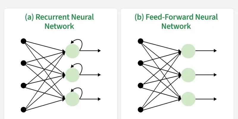
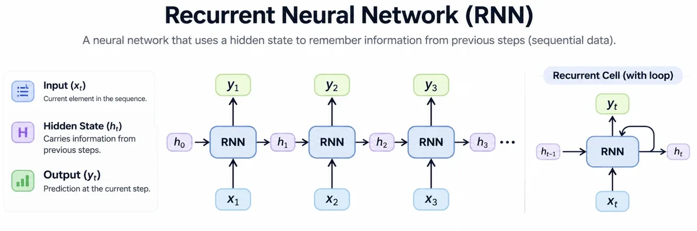
That memory is called the hidden state, written . It is just a vector of numbers. The update is surprisingly small:
is the input at step (for example a word vector), is the memory from the step before and the new memory. and are weight matrices and a bias. The same , and are used at every step. The squeezes the result into the range -1 to 1.
The output at each step is then a simple read-out of the state, , or you may only use the last state, for example to classify a whole sentence.
Time steps are not layers
This is the point beginners find hardest, so look at it twice. The diagram of an RNN usually shows several boxes in a row. They are not different layers. They are the same cell used again at every time step, with the same weights.
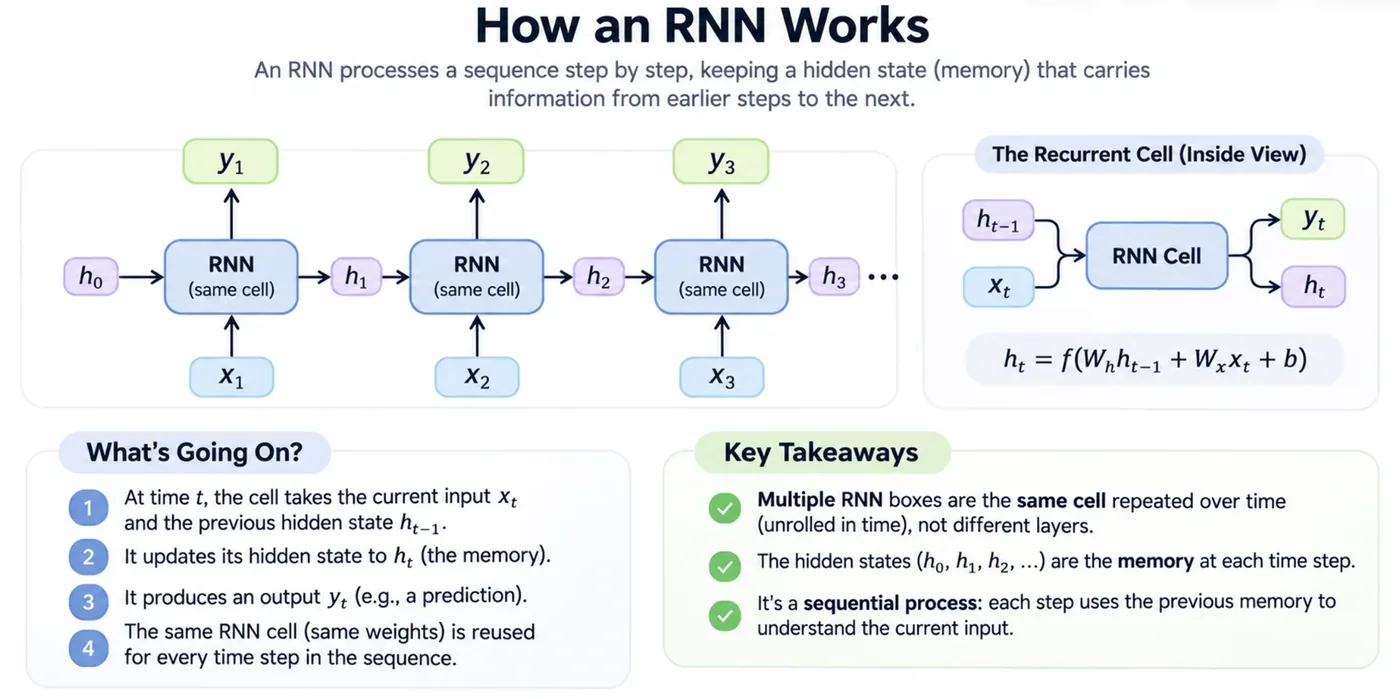
| Time steps | Layers | |
|---|---|---|
| What they process | Different elements of a sequence | Different depths of the network |
| Weights | The same ones, reused | Usually separate for each layer |
| Passes along | Hidden state, forward in time | Representations, up the stack |
| Example | 10 words = 10 time steps | 2 stacked RNN layers |
One RNN layer can process 100 steps, and still have the same number of parameters as when processing 4.
Compute it by hand
Take the sentence "I love machine learning". Each word becomes a small vector. Before the first word the memory is all zeros. Each step reads one word and updates the memory.
import numpy as np
import torch
import torch.nn as nn

rng = np.random.default_rng(0)
words = ["I", "love", "machine", "learning"]
x = rng.normal(size=(4, 3))                    # each word is a vector of 3 numbers (an "embedding")
Wx = rng.normal(size=(3, 5)) * 0.5            # input -> hidden weights   (shared by every step)
Wh = rng.normal(size=(5, 5)) * 0.5            # hidden -> hidden weights  (shared by every step)
b = np.zeros(5)

h = np.zeros(5)                                # h0: the starting memory is empty
for t, word in enumerate(words, start=1):
    h = np.tanh(x[t - 1] @ Wx + h @ Wh + b)    # the SAME formula, the SAME weights, every time step
    print(f"t={t}  read '{word:8s}'  hidden state = {h.round(2)}")

# check against PyTorch's own RNN layer, loaded with the same weights
rnn = nn.RNN(input_size=3, hidden_size=5, batch_first=True)
with torch.no_grad():
    rnn.weight_ih_l0.copy_(torch.tensor(Wx.T)); rnn.weight_hh_l0.copy_(torch.tensor(Wh.T))
    rnn.bias_ih_l0.zero_(); rnn.bias_hh_l0.zero_()
    out, h_last = rnn(torch.tensor(x, dtype=torch.float32).unsqueeze(0))
print("\nmatches torch.nn.RNN:", np.allclose(h_last[0, 0].numpy(), h, atol=1e-5))
print("parameters in this one RNN layer:", sum(p.numel() for p in rnn.parameters()), "(the same count for 4 steps or 4,000)")t=1 read 'I ' hidden state = [-0.33 0.07 0.14 -0.01 -0.35]
t=2 read 'love ' hidden state = [-0.35 -0.22 -0.32 0.04 -0.2 ]
t=3 read 'machine ' hidden state = [-0.89 -0.33 -0.79 -0.27 0.52]
t=4 read 'learning' hidden state = [ 0.98 0.18 0.06 0.91 -0.76]
matches torch.nn.RNN: True
parameters in this one RNN layer: 50 (the same count for 4 steps or 4,000)The hidden state after step 1 summarises "I". After step 2 it reflects "I love", and after step 4 it holds a compressed trace of the whole sentence. The check at the bottom confirms that PyTorch's nn.RNN, given the same weights, produces identical numbers. And the last line is the important one: the layer has 50 parameters whether the sequence is 4 words or 4,000 long. That is why RNNs can handle inputs of any length.
Training: backpropagation through time
You train an RNN with the same recipe as before, forward pass, loss, backward pass, update, but the backward pass has a twist. To work out how an early word affected a late error, the gradient must travel backwards through every time step. This is called backpropagation through time (BPTT): unroll the loop into a long chain and run ordinary backpropagation on it.
Here is the catch, and it is the Session 8 problem all over again. The gradient flowing back from step to step is a product of one factor per step in between:
Each factor contains the slope (at most 1, usually much less) times the weight matrix . Multiply dozens of these together and the result either shrinks towards zero (vanishing gradient) or grows without bound (exploding gradient), depending on whether makes things smaller or bigger.
Measure it directly. We run an untrained RNN over 60 steps and ask how much each earlier input still influences the final output:
import matplotlib.pyplot as plt
import torch
import torch.nn as nn

torch.manual_seed(0)
T = 60
rnn = nn.RNN(1, 32, batch_first=True)          # untrained, default start
x = torch.randn(1, T, 1, requires_grad=True)
out, _ = rnn(x)
out[0, -1].sum().backward()                    # the loss depends on the LAST step only
grad = x.grad[0, :, 0].abs()                   # how much does each input position influence it?

for t in (T - 1, T - 5, T - 10, T - 20, T - 40, 0):
    print(f"influence of the input {T - 1 - t:2d} steps back: {grad[t].item():.2e}")

fig, ax = plt.subplots(figsize=(6.4, 3.6))
ax.semilogy(range(T), grad.numpy() + 1e-30, lw=2, color="#DC2626")
ax.set_xlabel("position in the sequence (the last step is on the right)"); ax.set_ylabel("gradient size (log)")
ax.spines[["top", "right"]].set_visible(False)
fig.tight_layout()influence of the input 0 steps back: 2.67e-01
influence of the input 4 steps back: 5.41e-02
influence of the input 9 steps back: 5.12e-03
influence of the input 19 steps back: 3.20e-05
influence of the input 39 steps back: 1.67e-09
influence of the input 59 steps back: 9.00e-14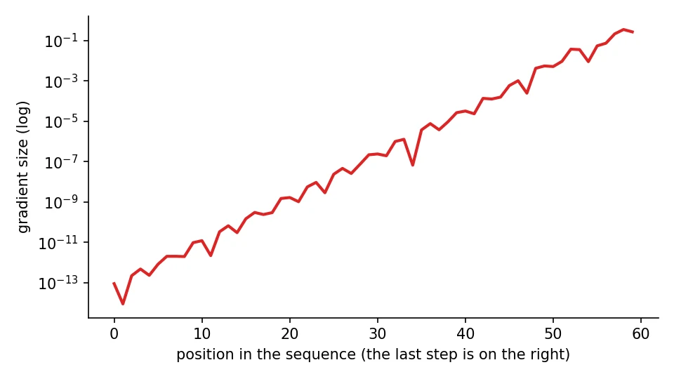
The influence of the very last input is 0.27. Ten steps back it is 0.005. Twenty steps back, 0.00003. Forty steps back, 0.0000000017 and at the start, 0.00000000000009. The signal drops by roughly thirteen orders of magnitude across 60 steps. A learning signal that small is the same as none. The network cannot connect a word at the start of a paragraph to an error at the end.
The memory test
Let's turn that into a measurable experiment. The task: a sequence of random numbers, and the label is whether the first number was positive. Everything after it is noise. To solve it the RNN must carry one bit of information across the whole sequence. We train for 500 steps, three times with different random starts, at four sequence lengths:
import torch
import torch.nn as nn

# The task: the label is the sign of the FIRST number. Everything after it is noise.
def make_batch(batch, T):
    x = torch.randn(batch, T, 1)
    y = (x[:, 0, 0] > 0).float()
    return x, y

class Net(nn.Module):
    def __init__(self):
        super().__init__()
        self.rnn = nn.RNN(1, 32, batch_first=True)
        self.head = nn.Linear(32, 1)
    def forward(self, x):
        _, h = self.rnn(x)                       # h: the memory after reading the whole sequence
        return self.head(h[0]).squeeze(-1)

print("sequence length   accuracy of a plain RNN (mean of 3 runs)   (50% = pure guessing)")
for T in (5, 15, 30, 60):
    accs = []
    for seed in range(3):                                # three different random starts
        torch.manual_seed(seed)
        net = Net(); opt = torch.optim.Adam(net.parameters(), lr=0.01)
        for step in range(500):
            x, y = make_batch(64, T)
            loss = nn.functional.binary_cross_entropy_with_logits(net(x), y)
            opt.zero_grad(); loss.backward()
            nn.utils.clip_grad_norm_(net.parameters(), 1.0)
            opt.step()
        x, y = make_batch(2000, T)
        accs.append(((net(x) > 0).float() == y).float().mean().item())
print(f"{T:10d} {sum(accs) / 3:.3f} (runs: {', '.join(f'{a:.2f}' for a in accs)})")sequence length accuracy of a plain RNN (mean of 3 runs) (50% = pure guessing)
5 0.994 (runs: 1.00, 0.99, 1.00)
15 0.963 (runs: 0.99, 0.92, 0.98)
30 0.715 (runs: 0.55, 0.64, 0.95)
60 0.507 (runs: 0.49, 0.53, 0.50)The accuracy falls as the sequence gets longer: 0.994 at 5 steps, 0.963 at 15, 0.715 at 30 and 0.507 at 60, which is no better than a coin flip. Look at the individual runs at length 30 (0.55, 0.64, 0.95). Sometimes the network finds a trick and sometimes it does not, which shows how fragile this is. A plain RNN has a short memory.
In an RNN processing a 50-word sentence, how many separate sets of weights does the recurrent layer have?
What RNNs are good at
Despite the memory limit, RNNs were the standard tool for sequences for years. They handle these shapes of problem:
- Many-to-one: read a whole sequence, give one answer (sentiment of a review, classify a sensor trace).
- One-to-many: one input, a sequence out (describe an image with a caption).
- Many-to-many: sequence in, sequence out (translation, speech to text, tagging each word).
Typical applications: predicting the next word or character, machine translation, speech recognition, music generation, stock and weather forecasting and analysing gene sequences.
A character-level language model
Here is a small, complete example. The model reads text one character at a time and learns to predict the next character. We train it on a few English proverbs and then let it generate text, feeding each predicted character back as the next input:
import torch
import torch.nn as nn

text = ("practice makes perfect. slow and steady wins the race. a stitch in time saves nine. "
        "well begun is half done. knowledge is power. patience is a virtue. ") * 6
chars = sorted(set(text)); idx = {c: i for i, c in enumerate(chars)}
data = torch.tensor([idx[c] for c in text])
print(f"{len(text)} characters, {len(chars)} different symbols")

class CharRNN(nn.Module):
    def __init__(self, vocab, hidden=96):
        super().__init__()
        self.emb = nn.Embedding(vocab, 24); self.rnn = nn.RNN(24, hidden, batch_first=True); self.out = nn.Linear(hidden, vocab)
    def forward(self, x, h=None):
        y, h = self.rnn(self.emb(x), h)
        return self.out(y), h

torch.manual_seed(0)
model = CharRNN(len(chars)); opt = torch.optim.Adam(model.parameters(), lr=0.01)
seq = 40
for step in range(1, 501):
    starts = torch.randint(0, len(data) - seq - 1, (64,))
    x = torch.stack([data[s:s + seq] for s in starts]); y = torch.stack([data[s + 1:s + seq + 1] for s in starts])
    logits, _ = model(x)
    loss = nn.functional.cross_entropy(logits.reshape(-1, len(chars)), y.reshape(-1))
    opt.zero_grad(); loss.backward(); nn.utils.clip_grad_norm_(model.parameters(), 1.0); opt.step()
    if step in (1, 50, 200, 500):
        print(f"step {step:3d}   loss {loss.item():.3f}")

# generate: feed the model its own output one character at a time
model.eval(); c = torch.tensor([[idx["p"]]]); h = None; out = ["p"]
with torch.no_grad():
    for _ in range(150):
        logits, h = model(c, h)
        c = torch.multinomial(torch.softmax(logits[0, -1] / 0.7, dim=0), 1).view(1, 1)
        out.append(chars[c.item()])
print("\ngenerated:", "".join(out))906 characters, 24 different symbols
step 1 loss 3.199
step 50 loss 0.078
step 200 loss 0.065
step 500 loss 0.056
generated: patience is a virtue. practice makes perfect. slow and steady wins the race. a stitch in time saves nine. well begun is half done. knowledge is power.The loss falls from 3.2 (guessing among 24 symbols) to 0.056 in 500 steps, and the model reproduces the proverbs. Be honest about what this shows: the training text is tiny and repeated six times, so the network has largely memorised it. It is a demonstration of the mechanism (read a character, update the memory, predict the next one), not of understanding. The same loop, scaled up enormously and with a better architecture, is the idea behind language models.
The simple recurrent network was popularised by Jeffrey Elman in 1990. By 2016, Google Translate had moved to a neural system built on recurrent layers (LSTMs), which Google reported reduced translation errors by 55 to 85 percent on several language pairs.Elman, 1990; Google Research blog on GNMT, 2016
Forecasting a time series
RNNs can also forecast. We create a made-up daily series with a yearly cycle, a slow upward trend and noise (think average temperature), cut it into windows of 30 days, and train the RNN to predict the next day.
import numpy as np
import matplotlib.pyplot as plt
import torch
import torch.nn as nn

# A made-up daily series with a yearly cycle, a slow trend and noise (think: average daily temperature)
rng = np.random.default_rng(1)
t = np.arange(1500)
series = 25 + 10 * np.sin(2 * np.pi * t / 365) + 0.004 * t + rng.normal(0, 1.5, len(t))
series = (series - series.mean()) / series.std()

def make_windows(s, seq_len):
    X = np.array([s[i:i + seq_len] for i in range(len(s) - seq_len)])
    y = s[seq_len:]
    return X[..., None], y                    # X shape: (samples, seq_len, 1)

seq_len, split = 30, 1100
X, y = make_windows(series, seq_len)
X_tr, y_tr, X_te, y_te = [torch.tensor(a, dtype=torch.float32) for a in (X[:split], y[:split], X[split:], y[split:])]

class Forecaster(nn.Module):
    def __init__(self):
        super().__init__(); self.rnn = nn.RNN(1, 32, batch_first=True); self.head = nn.Linear(32, 1)
    def forward(self, x):
        _, h = self.rnn(x); return self.head(h[0]).squeeze(-1)

torch.manual_seed(0)
model = Forecaster(); opt = torch.optim.Adam(model.parameters(), lr=0.005)
for epoch in range(40):
    perm = torch.randperm(len(X_tr))
    for i in range(0, len(perm), 64):
        b = perm[i:i + 64]
        loss = nn.functional.mse_loss(model(X_tr[b]), y_tr[b]); opt.zero_grad(); loss.backward(); opt.step()

with torch.no_grad():
    pred = model(X_te)
mse = lambda a: ((a - y_te) ** 2).mean().item()
print(f"RNN test MSE            : {mse(pred):.3f}")
print(f"'same as yesterday' MSE : {mse(X_te[:, -1, 0]):.3f}   <- the baseline every model must beat")

fig, ax = plt.subplots(figsize=(8.2, 3.4))
ax.plot(y_te[:120].numpy(), color="#9CA3AF", lw=2, label="actual"); ax.plot(pred[:120].numpy(), color="#2563EB", lw=2, label="RNN prediction")
ax.set_xlabel("day (test period)"); ax.set_ylabel("standardised value"); ax.legend(frameon=False); ax.spines[["top", "right"]].set_visible(False)
fig.tight_layout()RNN test MSE : 0.071
'same as yesterday' MSE : 0.104 <- the baseline every model must beat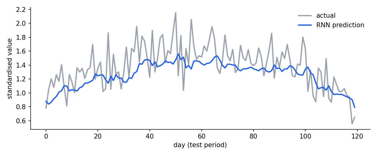
Always compare against the naive baseline of "tomorrow equals today". It scores a squared error of 0.104. The RNN scores 0.071, clearly better, so it learned something real from the pattern. A forecasting model that cannot beat "same as yesterday" is not worth deploying.
Variants
- Vanilla RNN: the simple one above, fine for short dependencies.
- Bidirectional RNN: reads the sequence forwards and backwards, so each position sees both past and future. Great when the whole sentence is available (tagging names in a sentence), not usable for live prediction.
- Stacked RNN: several recurrent layers, each feeding the next.
- LSTM and GRU: gated cells built to fix the short memory. The next session.
import torch.nn as nn

rnn = nn.RNN(input_size=1, hidden_size=50, batch_first=True)        # input shape: (batch, time steps, features)
# drop-in replacements with gates:
# nn.GRU(...)   nn.LSTM(...)   bidirectional=True for a bidirectional layer

out, h_last = rnn(x)      # out: the hidden state at every step; h_last: the final state
The wall of the plain RNN
We measured it twice: gradients shrink with distance and accuracy on a long-memory task falls to chance. Plain RNNs forget the beginning of a long sentence. Gradient clipping helps with exploding gradients, but vanishing ones need a change to the cell itself. That is what gates and a protected memory line provide in the next session.
Try it yourself
- In
remember_first.py, changenn.RNNtonn.GRUandnn.LSTM. What do you see at lengths 30 and 60? (Session 19 explains the surprises.) - In
gradient_through_time.py, changeT = 60to 200. How small does the influence of the first input get? - In
char_rnn.py, lower the temperature from 0.7 to 0.2 and then raise it to 1.5. How does the generated text change? - Add a
nn.RNNlayer withbidirectional=Trueto the forecaster. Does it make sense to use one for forecasting?
What comes next
Next we fix the memory. Session 19 introduces the LSTM, a recurrent cell with a protected memory line and three gates that decide what to keep, write and read.
Frequently asked questions
What is a recurrent neural network?
An RNN is a neural network for sequences. It reads the input one step at a time and passes a hidden state, a vector that acts as memory, from each step to the next. The same weights are used at every step, so it can handle sequences of any length.
What is the hidden state in an RNN?
The hidden state is the network's memory at a given time step: a vector computed from the current input and the previous hidden state. After reading a sentence, the final hidden state is a compressed summary of everything the network saw.
What is backpropagation through time?
BPTT is how RNNs are trained. The network is unrolled across the time steps into a long chain, and ordinary backpropagation runs backwards through the whole chain, so the weights are updated using the error at every step.
Why do RNNs struggle with long sequences?
During backpropagation through time the gradient is multiplied by a factor at every step. These factors are usually smaller than one, so the gradient from distant steps shrinks to almost nothing. The network cannot learn to connect early inputs to later errors, which is the vanishing gradient problem.
Are RNNs still used today?
Less than before. Transformers replaced them for most language tasks, but RNN-style models are still used for some time-series, speech and on-device tasks, and newer state-space and recurrent designs have revived interest in the idea.