The Vanishing Gradient Problem and Learning-Rate Decay, Explained with Real Numbers

Imagine passing a message down a line of twenty people, and each person whispers it at a quarter of the volume they heard. By the time it reaches the far end, nobody can hear anything. That is the vanishing gradient problem, and for years it stopped researchers from training deep neural networks at all.

This session explains where the problem comes from, shows it happening in real numbers, lists the standard fixes, and then covers its sibling: how to lower the learning rate as training goes on so the model settles gently instead of bouncing. It builds directly on the activation functions of Session 6 and the optimisation loop of Session 7.

Where the vanishing comes from

Training a network needs the gradient of the loss with respect to every weight, including the ones in the very first layer. The method for getting them, backpropagation (Session 10), works backwards from the output and uses the chain rule: the gradient for an early layer is a product of one slope per layer that sits between it and the output.

Now remember what we found in Session 6: the slope of the sigmoid is at most 0.25. Multiply a handful of numbers that are each at most 0.25 and watch what happens:

# The chain rule multiplies one slope per layer. The biggest slope sigmoid ever has is 0.25.
for layers in (3, 5, 10, 20):
    print(f"{layers:2d} layers: 0.25 ** {layers:2d} = {0.25 ** layers:.2e}")
print("\nwith ReLU the slope is exactly 1 for positive inputs: 1 ** 20 =", 1 ** 20)

 3 layers: 0.25 **  3 = 1.56e-02
 5 layers: 0.25 **  5 = 9.77e-04
10 layers: 0.25 ** 10 = 9.54e-07
20 layers: 0.25 ** 20 = 9.09e-13

with ReLU the slope is exactly 1 for positive inputs: 1 ** 20 = 1

Three layers is fine. Ten layers gives a gradient a million times smaller than the one at the output. Twenty layers gives 0.0000000000009. The early layers get an almost zero learning signal, so their weights barely move and they stay close to their random starting values. The loss stops improving even though training keeps running. That is the vanishing gradient.

It is worst in very deep networks, and in recurrent networks that are "unrolled" over many time steps (Session 18), where the same multiplication happens along the length of a sentence.

Measuring it for real

Let's not just argue it. We build a 20-layer network twice, once with sigmoid activations and once with ReLU, run one backward pass and measure how big the gradient is in every layer.

import torch
import torch.nn as nn
import matplotlib.pyplot as plt

def grad_norms(activation, depth=20, width=32, seed=0):
    torch.manual_seed(seed)
    layers = []
    for _ in range(depth):
        lin = nn.Linear(width, width)
        nn.init.xavier_normal_(lin.weight)                    # a sensible, standard initialisation
        layers += [lin, activation()]
    net = nn.Sequential(*layers, nn.Linear(width, 1))
    x = torch.randn(64, width); y = torch.randn(64, 1)
    nn.MSELoss()(net(x), y).backward()                        # one backward pass
    return [m.weight.grad.norm().item() for m in net if isinstance(m, nn.Linear)][:-1]   # per hidden layer

sig, relu = grad_norms(nn.Sigmoid), grad_norms(nn.ReLU)
print("gradient norm in the LAST hidden layer  :  sigmoid {:.2e}   ReLU {:.2e}".format(sig[-1], relu[-1]))
print("gradient norm in the FIRST hidden layer :  sigmoid {:.2e}   ReLU {:.2e}".format(sig[0], relu[0]))
print("first / last ratio                      :  sigmoid {:.1e}   ReLU {:.1e}".format(sig[0] / sig[-1], relu[0] / relu[-1]))

fig, ax = plt.subplots(figsize=(6.6, 3.8))
ax.semilogy(range(1, 21), sig, "-o", ms=4, lw=2, color="#DC2626", label="sigmoid")
ax.semilogy(range(1, 21), relu, "-o", ms=4, lw=2, color="#16A34A", label="ReLU")
ax.set_xlabel("layer (1 = closest to the input)"); ax.set_ylabel("gradient size (log scale)")
ax.set_xticks(range(1, 21, 2)); ax.legend(frameon=False); ax.spines[["top", "right"]].set_visible(False)
fig.tight_layout()

gradient norm in the LAST hidden layer  :  sigmoid 1.24e-01   ReLU 1.76e-02
gradient norm in the FIRST hidden layer :  sigmoid 2.02e-13   ReLU 3.64e-04
first / last ratio                      :  sigmoid 1.6e-12   ReLU 2.1e-02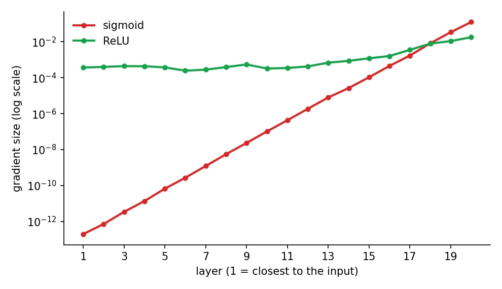

The numbers are stark. In the last hidden layer, sigmoid's gradient is 0.124. In the first hidden layer, it is 0.0000000000002, a drop of twelve orders of magnitude. With ReLU, the gradient in the first layer is 0.000364, about 2 percent of the last layer's. Still smaller, but alive and usable. (Both networks use Xavier initialisation, a sensible default, so this is not a case of a badly set up experiment.)

The opposite problem: exploding gradients

If the multiplied factors are bigger than 1, the product grows exponentially instead of shrinking. Weights jump wildly, the loss becomes NaN, and training dies in a different way. Here is a network with oversized weights:

import torch
import torch.nn as nn

torch.manual_seed(1)
# a deliberately unstable stack: big weights make gradients grow layer after layer
net = nn.Sequential(*[nn.Linear(16, 16) for _ in range(12)], nn.Linear(16, 1))
for m in net:
    if isinstance(m, nn.Linear):
        nn.init.normal_(m.weight, std=0.9)

x, y = torch.randn(32, 16), torch.randn(32, 1)
nn.MSELoss()(net(x), y).backward()

total = torch.sqrt(sum((p.grad ** 2).sum() for p in net.parameters()))
print(f"gradient norm before clipping: {total.item():.2e}")
torch.nn.utils.clip_grad_norm_(net.parameters(), max_norm=1.0)       # cap it
total = torch.sqrt(sum((p.grad ** 2).sum() for p in net.parameters()))
print(f"gradient norm after clipping : {total.item():.2f}")

gradient norm before clipping: 2.04e+14
gradient norm after clipping : 1.00

The gradient norm before clipping is about 200 trillion. Gradient clipping rescales the whole gradient so that its length never exceeds a chosen maximum. After clipping, it is exactly 1.00. The direction is preserved, only the size is tamed.

The standard fixes

No single cure, but a toolbox. Modern networks use several at once.

1. ReLU (or Leaky ReLU) in hidden layers. Its slope is exactly 1 for positive inputs, so the product does not shrink. This alone made much deeper networks trainable.
2. Careful weight initialisation. Starting weights too large or too small makes the problem worse from step one. Xavier (Glorot) initialisation suits sigmoid and tanh. He initialisation is designed for ReLU. They choose the starting variance so that signals keep roughly the same size layer after layer.
3. Batch normalisation. Re-centres and rescales each layer's inputs during training so they stay in a healthy range.
4. Residual (skip) connections. Give the gradient a shortcut that skips layers, so it has a direct path back to the early ones. This is what made 100-layer networks practical, and the same trick runs through every Transformer (Session 20).
5. Gradient clipping. A safety cap against explosions.
6. Gated architectures such as the LSTM, built specifically for long sequences (Session 19).

import tensorflow as tf
from tensorflow.keras import layers, models

model = models.Sequential([
    layers.Input(shape=(20,)),
    layers.Dense(64, activation="relu", kernel_initializer="he_normal"),
    layers.BatchNormalization(),
    layers.Dense(64, activation="relu", kernel_initializer="he_normal"),
    layers.Dense(1, activation="sigmoid"),
])
model.compile(optimizer=tf.keras.optimizers.Adam(1e-3, clipnorm=1.0),
              loss="binary_crossentropy")

ReLU, He initialisation, batch normalisation and clipnorm together keep gradients healthy in a deep stack.

Learning-rate decay

Now the second half of the session. A learning rate that is right at the start is usually too big at the end. Early on, big steps cover distance. Near the bottom, big steps keep jumping over the minimum and the loss never settles. The fix is to start with a larger learning rate and reduce it as training proceeds.

Common schedules

Two more you will see: reduce on plateau (lower the rate only when validation loss stops improving) and warm-up (start tiny, ramp up for the first few epochs, then decay), which is standard when training Transformers because large models are fragile at the very start.

import numpy as np
import matplotlib.pyplot as plt

epochs = np.arange(0, 100)
lr0 = 0.1
step   = lr0 * 0.5 ** (epochs // 25)                       # halve every 25 epochs
expo   = lr0 * 0.95 ** epochs                              # multiply by 0.95 each epoch
cosine = 0.5 * lr0 * (1 + np.cos(np.pi * epochs / 100))    # glide down along a cosine
warm   = np.where(epochs < 10, lr0 * (epochs + 1) / 10, 0.5 * lr0 * (1 + np.cos(np.pi * (epochs - 10) / 90)))

fig, ax = plt.subplots(figsize=(6.6, 3.8))
for y, name, c in [(step, "step decay", "#2563EB"), (expo, "exponential", "#F59E0B"), (cosine, "cosine", "#16A34A"), (warm, "warm-up + cosine", "#7C3AED")]:
    ax.plot(epochs, y, lw=2, color=c, label=name)
ax.set_xlabel("epoch"); ax.set_ylabel("learning rate"); ax.legend(frameon=False); ax.spines[["top", "right"]].set_visible(False)
fig.tight_layout()
print("epoch 0 / 50 / 99")
for name, y in [("step", step), ("exponential", expo), ("cosine", cosine)]:
    print(f"{name:12s} {y[0]:.4f} / {y[50]:.4f} / {y[99]:.4f}")

epoch 0 / 50 / 99
step         0.1000 / 0.0250 / 0.0125
exponential  0.1000 / 0.0077 / 0.0006
cosine       0.1000 / 0.0500 / 0.0000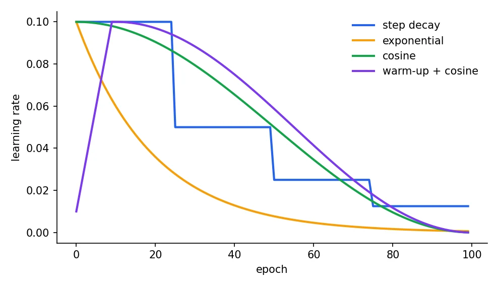

Does it actually help?

Here is a direct test. The same mini-batch gradient descent on the diabetes data, 60 epochs, once with a constant learning rate of 0.1 and once with that rate decayed by 5 percent each epoch.

import numpy as np
from sklearn.datasets import load_diabetes
from sklearn.preprocessing import StandardScaler

X, y = load_diabetes(return_X_y=True)
X = StandardScaler().fit_transform(X); y = (y - y.mean()) / y.std()
n = len(X)

def train(schedule, epochs=60, batch=16, seed=0):
    rng = np.random.default_rng(seed)
    w = np.zeros(X.shape[1]); history = []
    for epoch in range(epochs):
        lr = schedule(epoch)
        for i in range(0, n, batch):
            idx = rng.permutation(n)[:batch]
            w -= lr * (-2 * X[idx].T @ (y[idx] - X[idx] @ w) / len(idx))
        history.append(np.mean((y - X @ w) ** 2))
    last = np.array(history[-10:])
    return history[-1], last.std()

best = np.mean((y - X @ np.linalg.lstsq(X, y, rcond=None)[0]) ** 2)
print(f"best possible loss (exact solution): {best:.4f}\n")
print("schedule              final loss   wobble over last 10 epochs")
for name, sched in [("constant 0.1", lambda e: 0.1), ("decay 0.1 * 0.95^epoch", lambda e: 0.1 * 0.95 ** e)]:
    loss, wob = train(sched)
    print(f"{name:20s}  {loss:.4f}        {wob:.5f}")

best possible loss (exact solution): 0.4823

schedule              final loss   wobble over last 10 epochs
constant 0.1          0.5268        0.02249
decay 0.1 * 0.95^epoch  0.4847        0.00067

The exact least-squares solution has a loss of 0.4823, the best any line can do. With a constant learning rate the model ends at 0.5268, still wobbling (the loss varies by 0.022 over its last 10 epochs) because every noisy step is too big to settle. With decay it ends at 0.4847, within 0.0024 of the best possible, and the wobble drops to 0.0007. Same data, same model. Only the step size changed over time.

import torch

opt = torch.optim.Adam(model.parameters(), lr=1e-3)
sched = torch.optim.lr_scheduler.StepLR(opt, step_size=10, gamma=0.5)   # halve every 10 epochs
# alternative: ReduceLROnPlateau(opt, mode="min", factor=0.5, patience=3), then sched.step(val_loss)

for epoch in range(50):
    for xb, yb in train_loader:
        loss = loss_fn(model(xb), yb)
        opt.zero_grad(); loss.backward()
        torch.nn.utils.clip_grad_norm_(model.parameters(), max_norm=1.0)   # cap exploding gradients
        opt.step()
    sched.step()                                                           # decay the learning rate

Try it yourself

1. In vanishing.py, change depth=20 to 5 and then 40. At what depth does the sigmoid network become hopeless?
2. Swap nn.ReLU for nn.Tanh. Where does tanh land between sigmoid and ReLU?
3. In decay_effect.py, try a faster decay of 0.9 per epoch. Does it help or does the model stop learning too early?
4. Plot your own warm-up schedule: linear rise for 5 epochs and then step decay.

What comes next

We now know how a model is told it is wrong (loss), how it moves to fix that (gradient descent) and what can go wrong in deep stacks (vanishing and exploding gradients). In Session 9 we take a break from supervised learning to meet clustering, which learns without labels, and then lay out the anatomy of an artificial neural network.

Frequently asked questions