In 2017, eight researchers at Google published a paper with a confident title: Attention Is All You Need. It described a new network design, the Transformer, for machine translation. The paper reported better translation scores than anything before it, and trained its base model in about 12 hours on eight GPUs. Within a few years nearly every important language model, and many image and audio models, were Transformers. GPT, Claude, Gemini and LLaMA are all descendants of that one design.
This is the first session of Part V, Generative AI. We start by seeing why RNNs and LSTMs (Sessions 18 and 19) had to be replaced, and then build the Transformer piece by piece: tokens, embeddings, attention, positions, the full encoder-decoder, and how text is generated. Every idea is backed by code you can run, using the real GPT-2 model. If you remember only one sentence, make it this one: a Transformer is a token-prediction machine.
Why RNNs had to go
Recurrent networks read a sequence one token at a time. That caused three problems:
- They are slow. Step 50 cannot start until step 49 has finished, so a GPU's thousands of cores sit idle. Adding more GPUs stops helping.
- They forget. Even an LSTM squeezes the whole past into one fixed-size memory, and relationships between far-apart words get weaker (Session 19).
- Order is fragile. The model has to track word order step by step.
The Transformer's answer has three parts: process everything in parallel, let every token look directly at every other token (self-attention), and add word order back in with positional encoding.
Step 1: tokens and embeddings
A Transformer cannot read text. It reads numbers. So text is first cut into small pieces called tokens, and each token is given an integer ID from the model's vocabulary. The tokens are often whole words, but common practice uses subwords, so a rare word is built from familiar pieces. The popular algorithm for choosing the pieces is byte-pair encoding (BPE). Let's look at GPT-2's tokenizer:
from transformers import AutoTokenizer

tok = AutoTokenizer.from_pretrained("gpt2")                 # the tokenizer GPT-2 was trained with (byte-pair encoding)
for text in ["I love AI", "Tokenization is unbelievable", "السلام علیکم"]:
    ids = tok(text)["input_ids"]
    print(f"{text!r}")
    print("   tokens:", tok.convert_ids_to_tokens(ids))
    print("   ids   :", ids, f"({len(ids)} tokens for {len(text)} characters)")

print("\nvocabulary size:", tok.vocab_size)'I love AI'
tokens: ['I', 'Ġlove', 'ĠAI']
ids : [40, 1842, 9552] (3 tokens for 9 characters)
'Tokenization is unbelievable'
tokens: ['Token', 'ization', 'Ġis', 'Ġunbelievable']
ids : [30642, 1634, 318, 24479] (4 tokens for 28 characters)
'السلام علیکم'
tokens: ['اÙĦ', 'س', 'ÙĦ', 'ا', 'Ùħ', 'ĠØ', '¹', 'ÙĦ', 'Û', 'Į', 'Ú', '©', 'Ùħ']
ids : [23525, 45692, 13862, 12919, 25405, 17550, 117, 13862, 151, 234, 150, 102, 25405] (13 tokens for 12 characters)
vocabulary size: 50257"I love AI" is 3 tokens with IDs 40, 1842 and 9552. The Ġ is how this tokenizer marks a leading space. "Tokenization is unbelievable" becomes 4 tokens, with "Tokenization" split into Token and ization. And look at the Urdu line: 13 tokens for 12 characters. This older tokenizer was trained mostly on English, so a language it saw less of is cut into tiny fragments. That costs more compute and more money per sentence, and it is one reason newer tokenizers include far more multilingual text.
Next, each token ID is turned into a vector by looking it up in an embedding table. These vectors are learned, and tokens with related meanings end up close together:
import torch
from transformers import AutoModelForCausalLM, AutoTokenizer

tok = AutoTokenizer.from_pretrained("gpt2")
model = AutoModelForCausalLM.from_pretrained("gpt2").eval()      # GPT-2 small: a decoder-only Transformer

emb = model.transformer.wte                                      # the token-embedding lookup table
print("embedding table:", tuple(emb.weight.shape), "= (vocabulary size, vector length)")
ids = tok("I love AI", return_tensors="pt")["input_ids"][0]
print("token ids for 'I love AI':", ids.tolist())
print("vector of the first token, first 6 numbers:", emb(ids[0])[:6].detach().numpy().round(3))

# similar tokens sit close together (cosine similarity of the learned vectors)
def vec(word): return emb.weight[tok(" " + word)["input_ids"][0]].detach()
cos = lambda a, b: torch.cosine_similarity(vec(a), vec(b), dim=0).item()
print("\ncosine similarity:")
for a, b in [("king", "queen"), ("king", "banana"), ("Monday", "Tuesday"), ("Monday", "banana")]:
    print(f"   {a:7s} vs {b:7s} {cos(a, b):.2f}")

n_total = sum(p.numel() for p in model.parameters())
n_block = sum(p.numel() for p in model.transformer.h[0].parameters())
print(f"\ntotal parameters: {n_total:,}")
print(f"one Transformer block: {n_block:,}   x 12 blocks = {12 * n_block:,}")
print(f"token embeddings: {emb.weight.numel():,}")embedding table: (50257, 768) = (vocabulary size, vector length)
token ids for 'I love AI': [40, 1842, 9552]
vector of the first token, first 6 numbers: [ 0.147 -0.096 0.143 -0.106 -0.012 -0.096]
cosine similarity:
king vs queen 0.66
king vs banana 0.26
Monday vs Tuesday 0.89
Monday vs banana 0.28
total parameters: 124,439,808
one Transformer block: 7,087,872 x 12 blocks = 85,054,464
token embeddings: 38,597,376GPT-2's table has 50,257 rows (the vocabulary) and 768 columns, one 768-number vector per token. Notice the cosine similarities: "Monday" and "Tuesday" score 0.89, while "Monday" and "banana" score 0.28. Nobody told the model that days of the week go together. It learned it from text. The last lines show the whole model: 124,439,808 parameters, of which about 7.1 million sit in each of 12 identical Transformer blocks. That is the "small" GPT-2.
The base Transformer in the 2017 paper was trained in about 12 hours on eight NVIDIA P100 GPUs and set a new best score on English-to-German translation (28.4 BLEU). RNN-based systems of the time took far longer to train.Vaswani et al., Attention Is All You Need, 2017
Step 2: self-attention, the core idea
Read the sentence "The animal didn't cross the street because it was too tired". To understand "it" you have to look back at "animal". A good model needs each word to look at the other words and decide which ones matter. That is attention.
The mechanism works like a search engine inside the model. Every token creates three vectors from its embedding:
- a Query (Q): "what am I looking for?"
- a Key (K): "what do I contain?"
- a Value (V): "what will I hand over if I am picked?"
Each token's Query is compared with every token's Key, giving a relevance score. A softmax turns the scores into weights that sum to 1, and the output is the weighted average of the Values.
, and are matrices with one row per token. is every Query dotted with every Key, a table of "how much does token care about token ". is the length of a key vector. The softmax is applied to each row, so every token's attention weights add up to 1.
The , and vectors come from the token vectors by three learned weight matrices: , , . Here it is from scratch, for three tokens and tiny vectors:
import math
import numpy as np
import torch
import torch.nn.functional as F

rng = np.random.default_rng(0)
tokens, d = 3, 4                                  # three tokens ("I", "love", "AI"), 4 numbers per vector
x = rng.normal(size=(tokens, d))
Wq, Wk, Wv = (rng.normal(size=(d, d)) for _ in range(3))     # the learned projections
Q, K, V = x @ Wq, x @ Wk, x @ Wv

scores = Q @ K.T / math.sqrt(d)                   # how well each Query matches each Key
weights = np.exp(scores) / np.exp(scores).sum(axis=1, keepdims=True)     # softmax: each row sums to 1
out = weights @ V                                 # a weighted mix of the Values

print("attention weights (row = the token that is looking, column = the token it looks at):")
print(weights.round(2))
print("each row sums to:", weights.sum(axis=1).round(2))

# the decoder is not allowed to look ahead: mask the future with minus infinity before the softmax
mask = np.triu(np.ones((tokens, tokens), bool), k=1)
masked = np.where(mask, -np.inf, scores)
w2 = np.exp(masked) / np.exp(masked).sum(axis=1, keepdims=True)
print("\nwith the causal mask (no peeking at later tokens):")
print(w2.round(2))

ref = F.scaled_dot_product_attention(torch.tensor(Q)[None], torch.tensor(K)[None], torch.tensor(V)[None], is_causal=True)[0].numpy()
print("\nmatches PyTorch's built-in attention:", np.allclose(w2 @ V, ref))

# why divide by sqrt(d)? without it, big vectors give huge scores and the softmax saturates
print("\nvector length d    spread of raw scores    biggest softmax weight (unscaled)")
for dim in (4, 64, 512):
    q, k = rng.normal(size=(1, dim)), rng.normal(size=(50, dim))
    s = (q @ k.T)[0]
    p = np.exp(s - s.max()); p /= p.sum()
print(f"{dim:12d} {s.std():10.1f} {p.max():.2f}")attention weights (row = the token that is looking, column = the token it looks at):
[[0.38 0.3 0.32]
[0.32 0.21 0.47]
[0.05 0.01 0.94]]
each row sums to: [1. 1. 1.]
with the causal mask (no peeking at later tokens):
[[1. 0. 0. ]
[0.61 0.39 0. ]
[0.05 0.01 0.94]]
matches PyTorch's built-in attention: True
vector length d spread of raw scores biggest softmax weight (unscaled)
4 2.0 0.42
64 7.7 0.43
512 22.3 0.75Read the first table: row 3 (the token "AI") puts 0.94 of its attention on itself, while row 1 spreads its attention almost evenly. Each row sums to 1. The second table adds the causal mask, used by text-generating models: each token may only look at itself and earlier tokens, so the future is blocked (the upper triangle is zero). This stops the decoder from cheating by reading the answer it is supposed to predict.
Why divide by the square root of ?
The last table in that output is the reason for the . A dot product adds up products, so its typical size grows with the length of the vectors: the spread of raw scores goes from 2.0 (with ) to 7.7 (with ) to 22.3 (with ). Big scores make the softmax extremely peaky: at one token already takes 75 percent of the weight, and gradients through such a saturated softmax almost vanish (a familiar problem from Session 8). Dividing by keeps the scores at a steady scale.
Multi-head attention
One attention pattern is not enough. One head might track grammar, another which noun a pronoun refers to, another nearby words. Multi-head attention runs several attention computations in parallel, each with its own , , , and then joins their results:
is the number of heads (12 in GPT-2 small) and mixes the heads' outputs back to the model's width. Each head works in a smaller space (), so the total cost is about the same as one big head.
Step 3: putting back the word order
Attention treats its input as a set. Look at this check, which shuffles the tokens and compares the outputs:
import numpy as np
import matplotlib.pyplot as plt

def positional_encoding(n_positions, d):
    pos = np.arange(n_positions)[:, None]
    i = np.arange(d // 2)[None, :]
    angle = pos / (10000 ** (2 * i / d))
    pe = np.zeros((n_positions, d))
    pe[:, 0::2], pe[:, 1::2] = np.sin(angle), np.cos(angle)
    return pe

pe = positional_encoding(50, 64)
print("encoding of position 0, first 6 numbers:", pe[0, :6].round(2))
print("encoding of position 1, first 6 numbers:", pe[1, :6].round(2))

# why it is needed: attention alone cannot tell word order
rng = np.random.default_rng(0)
x = rng.normal(size=(4, 8))
Wq, Wk, Wv = (rng.normal(size=(8, 8)) for _ in range(3))
def self_attention(x):
    Q, K, V = x @ Wq, x @ Wk, x @ Wv
    s = Q @ K.T / np.sqrt(8); w = np.exp(s) / np.exp(s).sum(1, keepdims=True)
    return w @ V
perm = [2, 0, 3, 1]                                  # shuffle the "words"
same = np.allclose(self_attention(x)[perm], self_attention(x[perm]))
print("\nshuffle the tokens, and the outputs are the same ones, just shuffled:", same)
print("so without position information, 'dog bites man' and 'man bites dog' look alike to attention")

fig, ax = plt.subplots(figsize=(7, 3.4))
im = ax.imshow(pe, aspect="auto", cmap="RdBu_r"); ax.set_xlabel("embedding dimension"); ax.set_ylabel("position in the sequence")
fig.colorbar(im, ax=ax, fraction=0.03)
fig.tight_layout()encoding of position 0, first 6 numbers: [0. 1. 0. 1. 0. 1.]
encoding of position 1, first 6 numbers: [0.84 0.54 0.68 0.73 0.53 0.85]
shuffle the tokens, and the outputs are the same ones, just shuffled: True
so without position information, 'dog bites man' and 'man bites dog' look alike to attention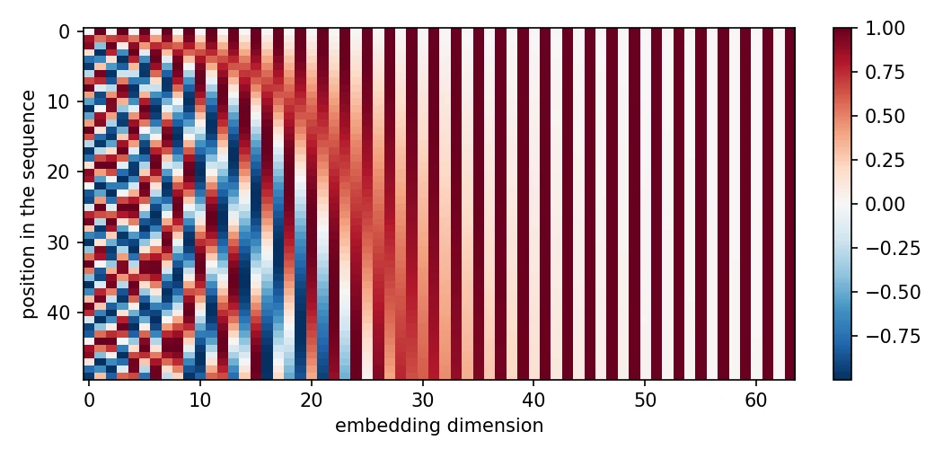
Shuffle the tokens and the outputs are the same ones, just shuffled. "Dog bites man" and "man bites dog" would look identical. So the Transformer adds position information to each embedding before attention. The original paper used fixed sine and cosine waves of different frequencies:
is the position of the token (0, 1, 2, ...), indexes pairs of dimensions and is the vector length. Low dimensions oscillate quickly and high dimensions slowly, like the second, minute and hour hands of a clock, so every position gets a unique pattern. The result is added to the token embedding.
Modern models often use other schemes (learned positions, rotary embeddings called RoPE, or ALiBi), but the job is the same: tell attention where each token sits.
Step 4: the rest of a block
A Transformer block is attention plus a few supporting parts, stacked many times:
- Residual connection ("Add"): the input of a sub-layer is added to its output, . It gives gradients a short path through deep stacks, the same idea as ResNet in Session 8.
- Layer normalisation ("Norm"): rescales each token's vector to a steady mean and spread so training stays stable.
- Feed-forward network: a small two-layer network applied to each token separately, to process what attention gathered. Typically it widens the vector by four times and uses a GELU or SwiGLU activation.
This is the original "post-norm" layout. Most modern models apply the normalisation before each sub-layer ("pre-norm"), which trains more stably in very deep stacks. The block is repeated times (12 in GPT-2 small).
The full encoder-decoder, with a translation example
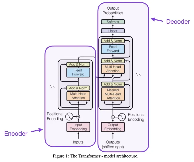
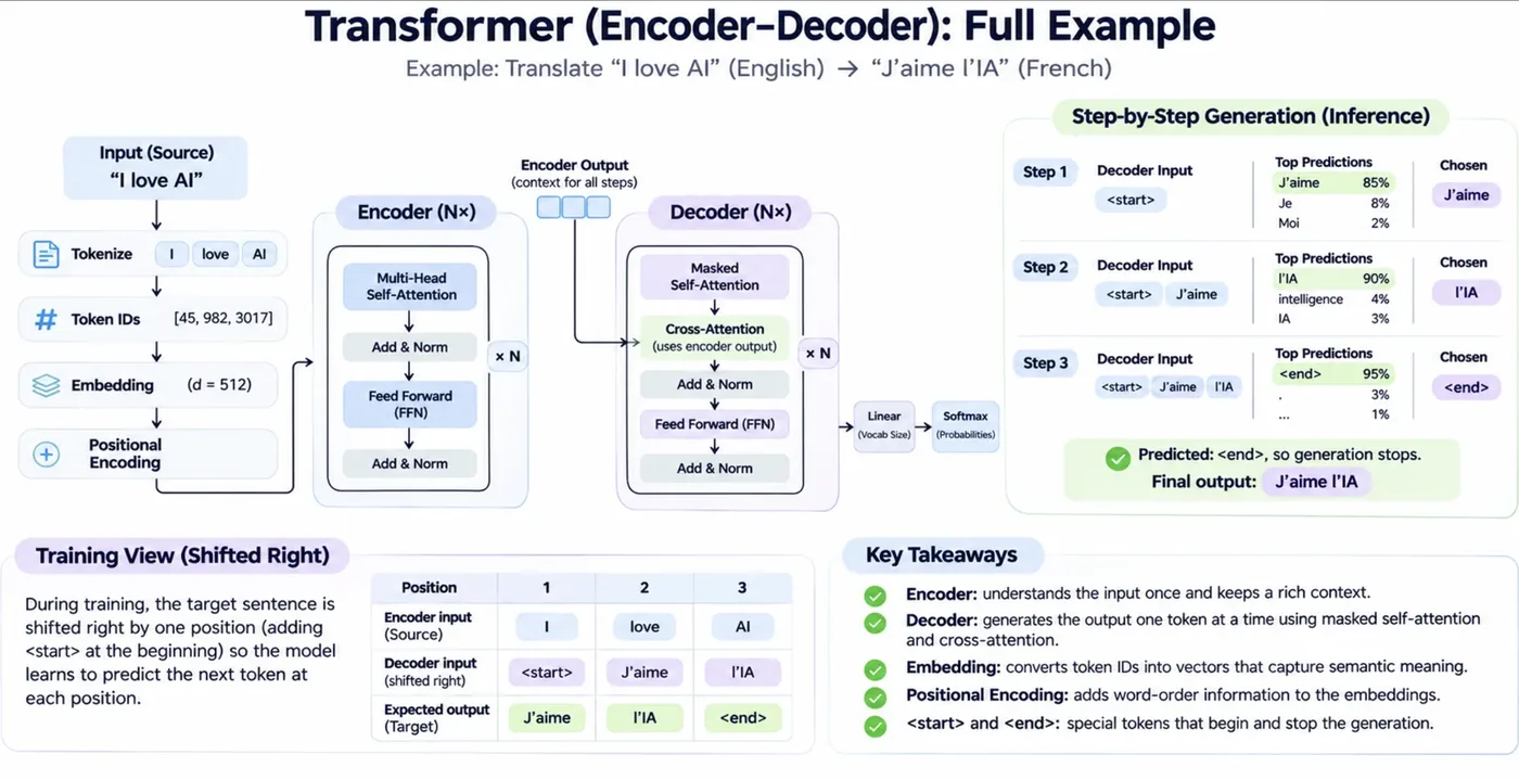
The original Transformer was built for translation, so it has two halves:
- The encoder reads the whole input at once and builds a rich representation of it.
- The decoder writes the output one token at a time. It has masked self-attention (so it cannot peek ahead), plus cross-attention: its Queries come from the output so far, while the Keys and Values come from the encoder, so it can look back at the input.
- At the very end, a linear layer turns the decoder's vector into one score (a logit) per vocabulary word, and a softmax turns them into probabilities.
Here is "I love AI" being translated into French, which the decoder writes one token at a time:
| Step | Decoder has so far | Decoder predicts next |
|---|---|---|
| 1 | <start> |
J'aime |
| 2 | <start> J'aime |
l'IA |
| 3 | <start> J'aime l'IA |
<end> |
At step 1, the output probabilities might look like J'aime 85 percent, Je 8 percent, Moi 2 percent, and cross-attention focuses on "I love". At step 2 it focuses on "AI", the part not yet translated. At step 3 <end> takes about 95 percent and generation stops. (These percentages are illustrative.)
Training: the target shifted right
During training we already know the correct answer, so we feed it all at once, shifted right by one position, and ask the model to predict each next token. The causal mask stops each position from seeing the answer it is predicting:
| Position | 1 | 2 | 3 |
|---|---|---|---|
| Encoder input | I | love | AI |
| Decoder input | <start> |
J'aime | l'IA |
| Expected output | J'aime | l'IA | <end> |
The loss is the cross-entropy from Session 6, averaged over positions. Feeding the true previous tokens during training, rather than the model's own guesses, is called teacher forcing.
Parallel or one at a time? Both are true
This trips up many beginners. We say Transformers process in parallel, and also that the decoder generates one token at a time. Both statements are correct.
- Parallel: reading the input (the encoder sees all tokens at once) and training (the whole target sentence goes in at once, with masking). This is where most of the compute goes, and it is why Transformers could be trained on enormous datasets.
- One at a time: generation at inference time. Token 3 depends on token 2, so it cannot exist before it. This is called autoregressive generation.
Three families of Transformers
- Encoder-decoder (the original, T5, BART): translation, summarisation.
- Encoder-only (BERT): understanding tasks such as classification, where the model reads a whole text.
- Decoder-only (GPT, LLaMA, Claude and most chat models): text generation. This is the design behind almost every modern LLM, and it is literally the next-token predictor described at the start.
Watching GPT-2 predict the next token
GPT-2 is a decoder-only Transformer, so it has one job: given the tokens so far, give a probability to every possible next token. Let's ask it:
import torch
from transformers import AutoModelForCausalLM, AutoTokenizer

tok = AutoTokenizer.from_pretrained("gpt2")
model = AutoModelForCausalLM.from_pretrained("gpt2").eval()

prompt = "The capital of Pakistan is"
ids = tok(prompt, return_tensors="pt")
with torch.no_grad():
    logits = model(**ids).logits[0, -1]                  # a score for every one of the 50,257 tokens
probs = torch.softmax(logits, dim=0)

print(f"prompt: {prompt!r}\n")
print("the model's five most likely next tokens:")
for p, i in zip(*torch.topk(probs, 5)):
    print(f"   {tok.decode(i)!r:14s} {p.item():6.1%}")

def entropy(p): return -(p * torch.log(p + 1e-12)).sum().item()
print("\neffect of temperature on the same scores:")
for T in (0.2, 1.0, 2.0):
    p = torch.softmax(logits / T, dim=0)
    print(f"   temperature {T}: top token gets {p.max().item():6.1%}, entropy {entropy(p):.2f}")

p = probs.sort(descending=True)
cum = p.values.cumsum(0)
print("\ntokens needed to cover 90% of the probability (top-p = 0.9):", int((cum < 0.9).sum()) + 1, "of 50,257")prompt: 'The capital of Pakistan is'
the model's five most likely next tokens:
' the' 10.0%
' a' 5.5%
' Islamabad' 3.9%
' home' 3.5%
' now' 2.9%
effect of temperature on the same scores:
temperature 0.2: top token gets 93.4%, entropy 0.32
temperature 1.0: top token gets 10.0%, entropy 5.74
temperature 2.0: top token gets 0.6%, entropy 9.32
tokens needed to cover 90% of the probability (top-p = 0.9): 1065 of 50,257For "The capital of Pakistan is", GPT-2 small puts 10.0 percent on " the", 5.5 percent on " a" and only 3.9 percent on " Islamabad". It is a small 2019 model, a good reminder that a language model predicts what text is likely, not what is true. The second part shows temperature: dividing the logits by before the softmax. At the top token gets 93.4 percent (predictable), at it gets 10.0 percent, and at only 0.6 percent (nearly random). The last line shows top-p (nucleus) sampling: 1,065 of 50,257 tokens cover 90 percent of the probability, so sampling can be limited to that set.
are the logits (raw scores). Low sharpens the distribution toward the top token, high flattens it. As this becomes greedy decoding.
import torch
from transformers import AutoModelForCausalLM, AutoTokenizer

tok = AutoTokenizer.from_pretrained("gpt2")
model = AutoModelForCausalLM.from_pretrained("gpt2").eval()
inputs = tok("Machine learning is", return_tensors="pt")

def show(title, **kw):
    torch.manual_seed(1)
    out = model.generate(**inputs, max_new_tokens=22, pad_token_id=tok.eos_token_id, **kw)
    print(f"{title}:\n   {tok.decode(out[0], skip_special_tokens=True)!r}\n")

show("greedy (always the top token)", do_sample=False)
show("sampling, temperature 0.8, top_p 0.9", do_sample=True, temperature=0.8, top_p=0.9)
show("sampling, temperature 1.5 (wilder)", do_sample=True, temperature=1.5)
show("beam search, 4 beams", do_sample=False, num_beams=4)greedy (always the top token):
"Machine learning is a very powerful tool for learning about the world around us. It's a tool that can help us understand the"
sampling, temperature 0.8, top_p 0.9:
"Machine learning is a huge part of the industry. As a result, I've been learning about it from people in my field"
sampling, temperature 1.5 (wilder):
"Machine learning is an extremely valuable aspect of deep learning for humans. Even though we don't typically see the problem in neuroscience so"
beam search, 4 beams:
"Machine learning is a great way to learn about the world around you, but it's also a great way to learn about the"Same model, same prompt, four decoding strategies. Greedy always takes the top token and is repetitive. Sampling with temperature 0.8 and top-p 0.9 gives varied, sensible text. Temperature 1.5 is wilder and starts drifting. Beam search keeps the best several partial sentences at each step and tends to give safe but repetitive output. Chat products typically sample with a moderate temperature.
GPT-2, released by OpenAI in 2019, came in four sizes. The one we used has 124 million parameters. The largest had 1.5 billion, which was considered dangerously capable at the time, and OpenAI initially held it back.OpenAI, Language Models are Unsupervised Multitask Learners, 2019
A look inside: an attention map
We can ask the real model what each token attended to. GPT-2 returns the attention weights of every layer and head:
import matplotlib.pyplot as plt
import torch
from transformers import AutoModelForCausalLM, AutoTokenizer

tok = AutoTokenizer.from_pretrained("gpt2")
model = AutoModelForCausalLM.from_pretrained("gpt2").eval()   # on newer transformers versions add attn_implementation="eager" to get attention weights
text = "The animal did not cross the street because it was too tired"
inputs = tok(text, return_tensors="pt")
with torch.no_grad():
    out = model(**inputs, output_attentions=True)

print("layers:", len(out.attentions), "| attention tensor per layer:", tuple(out.attentions[0].shape), "= (batch, heads, tokens, tokens)")
words = tok.convert_ids_to_tokens(inputs["input_ids"][0])
layer = 5
att = out.attentions[layer][0].mean(0)                      # average over the 12 heads of one layer
i = words.index("Ġit")
top = torch.topk(att[i], 3)
print(f"layer {layer + 1}, token 'it' looks most at:", [(words[j].lstrip('Ġ'), round(v.item(), 2)) for v, j in zip(top.values, top.indices)])

fig, ax = plt.subplots(figsize=(6.2, 5.2))
ax.imshow(att.numpy(), cmap="Blues")
labels = [w.lstrip("Ġ") for w in words]
ax.set_xticks(range(len(words)), labels, rotation=60, ha="right"); ax.set_yticks(range(len(words)), labels)
ax.set_xlabel("token being looked at"); ax.set_ylabel("token that is looking")
fig.tight_layout()layers: 12 | attention tensor per layer: (1, 12, 12, 12) = (batch, heads, tokens, tokens)
layer 6, token 'it' looks most at: [('The', 0.5), ('cross', 0.17), ('because', 0.1)]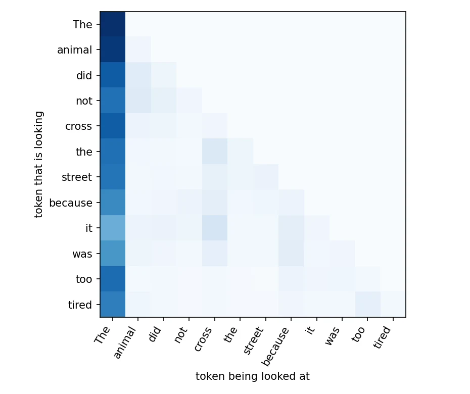
There are 12 layers, and each returns a tensor of shape (batch, 12 heads, 12 tokens, 12 tokens). The sentence is "The animal did not cross the street because it was too tired". We might hope that "it" attends to "animal". In this layer, averaged over heads, "it" looks mostly at "The" (0.50), then "cross" and "because". That is a real and well-known phenomenon called an attention sink: because the softmax forces weights to sum to 1, the model needs somewhere to park attention when nothing is especially relevant, and it often uses the first token. Different heads do different jobs, and one averaged map of one layer does not tell the whole story. Interpreting attention is harder than the neat diagrams in tutorials suggest.
The cost of attention
There is a price. Every token is compared with every other token, so the number of scores is for a sequence of tokens:
for n in (1_000, 8_000, 32_000, 128_000, 1_000_000):
    entries = n * n                                        # every token looks at every token
    gb = entries * 2 / 1e9                                 # 2 bytes per number (float16)
    print(f"{n:>9,} tokens -> {entries:>18,} attention scores per head per layer  (about {gb:,.2f} GB if stored in float16)")
print("\n10x longer text -> 100x more attention work: the cost grows with the SQUARE of the length") 1,000 tokens -> 1,000,000 attention scores per head per layer (about 0.00 GB if stored in float16)
8,000 tokens -> 64,000,000 attention scores per head per layer (about 0.13 GB if stored in float16)
32,000 tokens -> 1,024,000,000 attention scores per head per layer (about 2.05 GB if stored in float16)
128,000 tokens -> 16,384,000,000 attention scores per head per layer (about 32.77 GB if stored in float16)
1,000,000 tokens -> 1,000,000,000,000 attention scores per head per layer (about 2,000.00 GB if stored in float16)
10x longer text -> 100x more attention work: the cost grows with the SQUARE of the lengthAt 1,000 tokens that is a million scores per head per layer. At 128,000 tokens it is 16 billion, and storing them naively would take about 33 GB. Ten times more text costs a hundred times more attention work. Much of modern engineering (FlashAttention, sliding-window attention, grouped-query attention, a KV cache that stores each token's Keys and Values so they are not recomputed at every generation step) exists to tame this cost.
A glossary for what comes next
- Context window: the maximum number of tokens the model can see at once.
- Special tokens: reserved tokens such as
<start>,<end>,<pad>,[CLS]and[SEP]that carry structure. - Padding mask: hides the filler tokens that make sequences in a batch equal length.
- Hallucination: fluent but false output. The model predicts likely tokens, not verified facts.
- System prompt: hidden instructions placed before the user's message to set role and rules.
- Guardrails: checks before or after the model that block or correct unsafe or off-topic output.
- Scaling laws: performance improves predictably with more parameters, data and compute.
- Mixture of Experts (MoE): only a few specialised feed-forward "experts" run per token, so a huge model costs less per step.
- RLHF: tuning with human preferences so the model follows instructions (Session 13's bonus).
Why does the attention formula divide by the square root of d_k?
Transformers are called parallel, yet text generation is one token at a time. Which statement explains this?
Try it yourself
- In
tokens.py, tokenise your own name, a Roman-Urdu sentence and a line of code. Which one costs the most tokens per character? - In
next_token.py, change the prompt to "The largest city in Pakistan is". Does GPT-2 small know? What does that tell you about trusting an LLM? - In
generate.py, changetop_pto 0.3 and then 1.0. How does the style of the text change? - In
attention_map.py, trylayer = 0andlayer = 11. Do the maps look alike?
What comes next
Scale this decoder-only Transformer to billions of parameters, train it on a huge amount of text and you get a large language model. Session 21 covers how LLMs are built and trained, the model families, how to call one through an API, and what quantization and LoRA do.
Frequently asked questions
What is a Transformer in AI?
A Transformer is a neural network architecture, introduced by Google researchers in 2017, that processes a sequence by letting every token look at every other token through self-attention. It processes tokens in parallel, uses positional encoding to keep word order, and is the basis of GPT, Claude, Gemini, LLaMA and most modern language models.
What are Q, K and V in attention?
Each token produces a Query (what it is looking for), a Key (what it contains) and a Value (what it will contribute). The Query of one token is compared with the Keys of all tokens to get relevance weights, and the output is the weighted average of the Values.
Why do Transformers need positional encoding?
Self-attention treats its input as an unordered set, so on its own it cannot tell "dog bites man" from "man bites dog". Positional encodings add information about each token's position to its embedding so the model can use word order.
What is the difference between encoder-only, decoder-only and encoder-decoder models?
Encoder-only models like BERT read the whole input and are used for understanding tasks such as classification. Decoder-only models like GPT generate text one token at a time and power most chat models. Encoder-decoder models like T5 read an input and then generate a different output, as in translation.
Why is the Transformer's attention expensive for long texts?
Every token is compared with every other token, so the work grows with the square of the sequence length. Doubling the context makes attention about four times more expensive, which is why long-context models use techniques like FlashAttention and sliding-window attention.