
Show a photograph to the neural network from Session 9 and you hit two problems straight away. A small 28 by 28 picture is already 784 numbers, and a normal phone photo is millions. Connect every pixel to every neuron and you need tens of millions of weights before the network has learned anything. Worse, the network has no idea that neighbouring pixels belong together. Shuffle the pixels of an image and it cannot tell the difference.
A convolutional neural network (CNN) fixes both with one clever idea: look at small patches, and reuse the same patch-detector everywhere. This is the first session of Part IV, where networks are built to match the shape of their data. We will compute a convolution by hand, see what a network's first layer actually learns, and train a small CNN that reads handwritten digits at about 98.8 percent accuracy. You will want the training loop from Session 10 in mind.
The idea: slide a small filter over the image
An image is a grid of numbers (pixel brightness). To detect a pattern such as an edge, you do not need the whole image at once. You need a small window, say 3 by 3 pixels, that asks "is there a vertical edge here?". Slide that window across every position and you get a map of where the pattern appears.
- The window is called a kernel or filter: a small grid of learnable weights.
- Sliding it over the image and multiplying and adding at each spot is the convolution.
- The output grid is a feature map: it lights up wherever the filter's pattern is found.
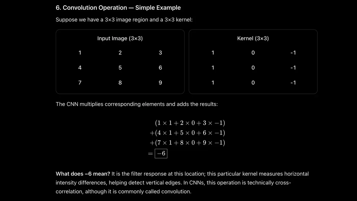
At each position the filter multiplies its weights by the pixels under it, element by element, and adds up the results:
is the image, the kernel and a bias. Strictly speaking this is cross-correlation (the kernel is not flipped as in textbook convolution), but every deep-learning library calls it convolution and, since the kernel is learned, the flip makes no difference.
Here is one convolution done by hand on a tiny 5 by 5 image with a classic vertical-edge detector, and then checked against PyTorch:
import numpy as np
import matplotlib.pyplot as plt
import torch
import torch.nn.functional as F
import torchvision

# --- one convolution, computed by hand ---
image = np.array([[1, 2, 0, 1, 3],
                  [0, 1, 3, 1, 0],
                  [2, 1, 0, 2, 1],
                  [1, 0, 2, 3, 1],
                  [0, 2, 1, 0, 2]], dtype=float)
kernel = np.array([[1, 0, -1],
                   [1, 0, -1],
                   [1, 0, -1]], dtype=float)          # a vertical-edge detector

out = np.zeros((3, 3))
for i in range(3):
    for j in range(3):
        patch = image[i:i + 3, j:j + 3]               # a 3x3 window of the image
        out[i, j] = (patch * kernel).sum()            # multiply element by element, then add up
print("feature map:\n", out)
print("top-left value by hand:", (image[:3, :3] * kernel).sum())

# the same thing with PyTorch (cross-correlation, which is what deep-learning libraries call convolution)
torch_out = F.conv2d(torch.tensor(image).view(1, 1, 5, 5), torch.tensor(kernel).view(1, 1, 3, 3))
print("matches PyTorch:", np.allclose(out, torch_out.numpy()[0, 0]))

# --- two hand-made filters on a real handwritten digit ---
digit = np.array(torchvision.datasets.MNIST("data", train=False, download=True)[0][0], dtype=float) / 255
vertical   = np.array([[-1, 0, 1], [-2, 0, 2], [-1, 0, 1]], dtype=float)
horizontal = vertical.T
conv = lambda k: F.conv2d(torch.tensor(digit).view(1, 1, 28, 28), torch.tensor(k).view(1, 1, 3, 3)).numpy()[0, 0]

fig, ax = plt.subplots(1, 3, figsize=(8.5, 3))
for a, img, t in zip(ax, [digit, np.abs(conv(vertical)), np.abs(conv(horizontal))], ["the image", "finds vertical edges", "finds horizontal edges"]):
    a.imshow(img, cmap="gray"); a.set_title(t, fontsize=10); a.axis("off")
fig.tight_layout()feature map:
[[ 0. 0. -1.]
[-2. -4. 3.]
[ 0. -2. -1.]]
top-left value by hand: 0.0
matches PyTorch: True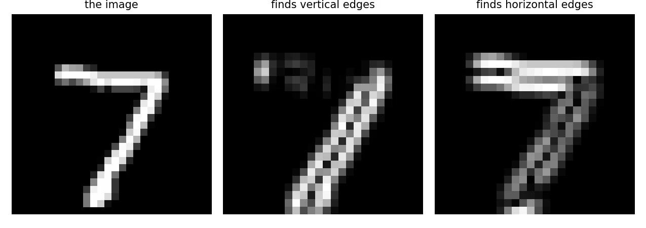
The kernel [[1, 0, -1], ...] says "bright on the left, dark on the right". The 3 by 3 feature map holds one number per window position, and the printout confirms that doing it by hand gives exactly what PyTorch computes. The figure then applies two fixed filters to a real handwritten digit. One lights up where the strokes are vertical, the other where they are horizontal.
The crucial step: in a CNN nobody designs these filters. Their nine numbers are parameters, learned by gradient descent like any other weight. And one set of nine numbers is reused at every position of the image, which is called weight sharing.
The idea that vision works in layers of local detectors comes from neuroscience. David Hubel and Torsten Wiesel studied the visual cortex of cats from 1959 and shared the 1981 Nobel Prize in Physiology or Medicine for it.Nobel Prize, 1981
Why this is so much cheaper
Compare the two designs for the first layer of a 28 by 28 digit network that produces 32 feature maps:
import torch
import torch.nn as nn

net = nn.Sequential(
    nn.Conv2d(1, 32, kernel_size=3), nn.ReLU(), nn.MaxPool2d(2),      # 28 -> 26 -> 13
    nn.Conv2d(32, 64, kernel_size=3), nn.ReLU(), nn.MaxPool2d(2),     # 13 -> 11 -> 5
    nn.Flatten(), nn.Linear(64 * 5 * 5, 64), nn.ReLU(), nn.Linear(64, 10),
)
x = torch.zeros(1, 1, 28, 28)                       # one grayscale 28x28 image
for layer in net:
    x = layer(x)
    n = sum(p.numel() for p in layer.parameters())
    print(f"{layer.__class__.__name__:10s} -> shape {tuple(x.shape)}   parameters {n:,}")
print("total parameters:", f"{sum(p.numel() for p in net.parameters()):,}")

# what a fully connected layer would need for just the FIRST layer's output
dense = 28 * 28 * (26 * 26 * 32)
print(f"\na dense layer making the same 26x26x32 output from the pixels would need {dense:,} weights")
print("the conv layer needs", 3 * 3 * 1 * 32 + 32, "(32 filters of 3x3, plus 32 biases)")Conv2d -> shape (1, 32, 26, 26) parameters 320
ReLU -> shape (1, 32, 26, 26) parameters 0
MaxPool2d -> shape (1, 32, 13, 13) parameters 0
Conv2d -> shape (1, 64, 11, 11) parameters 18,496
ReLU -> shape (1, 64, 11, 11) parameters 0
MaxPool2d -> shape (1, 64, 5, 5) parameters 0
Flatten -> shape (1, 1600) parameters 0
Linear -> shape (1, 64) parameters 102,464
ReLU -> shape (1, 64) parameters 0
Linear -> shape (1, 10) parameters 650
total parameters: 121,930
a dense layer making the same 26x26x32 output from the pixels would need 16,959,488 weights
the conv layer needs 320 (32 filters of 3x3, plus 32 biases)The convolutional first layer has 320 parameters (32 filters of 3 by 3, plus 32 biases). A fully connected layer making the same output from the same pixels would need 16,959,488 weights. That is more than 50,000 times as many. Look also at how the shape shrinks: 28 by 28 becomes 26 by 26 after the convolution, then 13 by 13 after pooling, and so on. The whole network has only 121,930 parameters, and 102,464 of them sit in the single dense layer near the end.
Stride, padding and the size of the output
Three dials control how the filter moves and what shape comes out:
- Stride: how many pixels the filter jumps each time. Stride 1 visits every position, stride 2 skips every other one and halves the output.
- Padding: adding a border of zeros around the image. Without it, the output shrinks, and border pixels are visited less often than centre pixels.
- Number of filters: each filter produces its own feature map, so 32 filters give 32 maps (the "depth" of the output).
is the input width (or height), the kernel size, the padding and the stride. Check it with the network above: , , , gives . With padding the output stays 28 ("same" padding).
is the number of input channels (1 for grayscale, 3 for RGB colour, or the number of feature maps from the previous layer) and the number of filters. Check: the second layer of our network has , matching the printout above. The count does not depend on the image size at all.
Pooling: shrink, keep the strongest
After a convolution, a pooling layer shrinks the feature maps. Max pooling looks at each small window (usually 2 by 2) and keeps only its largest value. The map gets 4 times smaller, so later layers are cheaper, and the network becomes a little less sensitive to the exact position of a feature.
import numpy as np

fmap = np.array([[1, 3, 2, 1],
                 [4, 6, 5, 2],
                 [7, 2, 9, 4],
                 [1, 8, 3, 6]])
pooled = fmap.reshape(2, 2, 2, 2).max(axis=(1, 3))          # max of each 2x2 block
print("4x4 feature map:\n", fmap)
print("\nafter 2x2 max pooling (2x2):\n", pooled)4x4 feature map:
[[1 3 2 1]
[4 6 5 2]
[7 2 9 4]
[1 8 3 6]]
after 2x2 max pooling (2x2):
[[6 5]
[8 9]]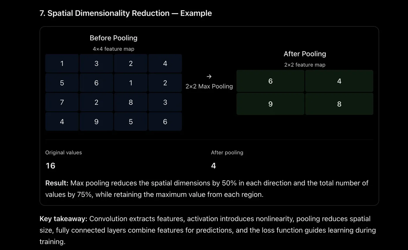
Average pooling takes the mean instead, and global average pooling averages each whole feature map into a single number, which many modern networks use in place of flattening.
The full CNN recipe
A typical CNN stacks a few blocks of convolution, ReLU, pooling, then flattens the maps into a vector and finishes with ordinary dense layers, as in Session 9:
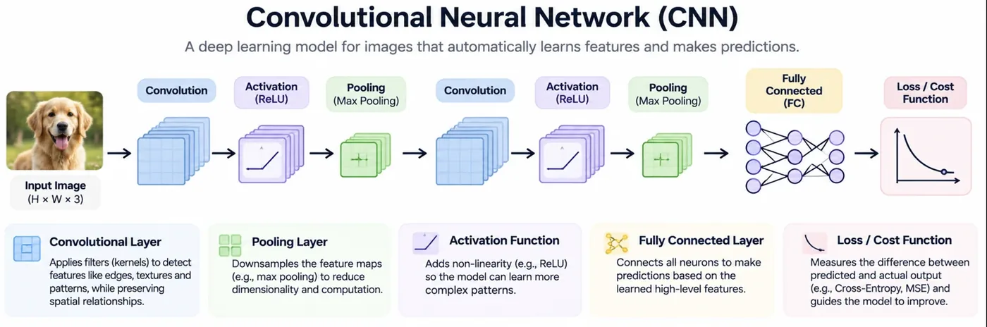
The early layers learn simple things like edges. Later layers combine edges into corners and textures, and later still into parts of objects. This hierarchy of features is learned, not designed, and it is the reason CNNs transformed computer vision.
Training a CNN on handwritten digits
Now the real thing. MNIST is the classic dataset: 60,000 training and 10,000 test images of handwritten digits, each 28 by 28 pixels. The network below has two convolution blocks and two dense layers (the same one we measured above). It trains for three passes through the data on an ordinary CPU.
import time
import matplotlib.pyplot as plt
import numpy as np
import torch
import torch.nn as nn
import torchvision
from torch.utils.data import DataLoader, TensorDataset

torch.manual_seed(0)
train = torchvision.datasets.MNIST("data", train=True, download=True)
test = torchvision.datasets.MNIST("data", train=False, download=True)
prep = lambda ds: ((ds.data.float() / 255 - 0.1307) / 0.3081).unsqueeze(1)      # scale, then standardise
X_tr, y_tr, X_te, y_te = prep(train), train.targets, prep(test), test.targets
loader = DataLoader(TensorDataset(X_tr, y_tr), batch_size=128, shuffle=True)

cnn = nn.Sequential(
    nn.Conv2d(1, 32, 3), nn.ReLU(), nn.MaxPool2d(2),
    nn.Conv2d(32, 64, 3), nn.ReLU(), nn.MaxPool2d(2),
    nn.Flatten(), nn.Linear(64 * 5 * 5, 64), nn.ReLU(), nn.Linear(64, 10),
)
opt = torch.optim.Adam(cnn.parameters(), lr=1e-3)
loss_fn = nn.CrossEntropyLoss()

def accuracy(model, X, y):
    model.eval()
    with torch.no_grad():
        return (model(X).argmax(1) == y).float().mean().item()

start = time.time()
for epoch in range(1, 4):
    cnn.train()
    for xb, yb in loader:
        loss = loss_fn(cnn(xb), yb)
        opt.zero_grad(); loss.backward(); opt.step()
    print(f"epoch {epoch}   last batch loss {loss.item():.3f}   test accuracy {accuracy(cnn, X_te, y_te):.4f}")
print(f"parameters: {sum(p.numel() for p in cnn.parameters()):,}")

# --- what did the first layer learn? ---
w = cnn[0].weight.detach().squeeze(1)                     # 32 filters of 3x3
fig, ax = plt.subplots(4, 8, figsize=(8, 4.2))
for a, f in zip(ax.ravel(), w):
    a.imshow(f, cmap="RdBu", vmin=-w.abs().max(), vmax=w.abs().max()); a.axis("off")
fig.suptitle("The 32 filters of the first layer", fontsize=11)
fig.tight_layout()

# --- and what does it see inside? ---
sample = X_te[:1]
with torch.no_grad():
    fm = cnn[1](cnn[0](sample))[0]                          # 32 feature maps after the first conv + ReLU
fig, ax = plt.subplots(3, 9, figsize=(9, 3.4))
ax[0, 0].imshow(sample[0, 0], cmap="gray")
for a in ax.ravel(): a.axis("off")
for a, m in zip(ax.ravel()[1:], fm[:26]):
    a.imshow(m, cmap="viridis")
fig.tight_layout()

# --- the mistakes it still makes ---
cnn.eval()
with torch.no_grad():
    pred = cnn(X_te).argmax(1)
wrong = (pred != y_te).nonzero().squeeze()[:12]
print("test images it got wrong:", int((pred != y_te).sum()), "of 10000")
fig, ax = plt.subplots(1, 12, figsize=(11, 1.6))
for a, i in zip(ax, wrong):
    a.imshow(test.data[i], cmap="gray"); a.set_title(f"{y_te[i].item()}→{pred[i].item()}", fontsize=9); a.axis("off")
fig.tight_layout()epoch 1 last batch loss 0.108 test accuracy 0.9808
epoch 2 last batch loss 0.013 test accuracy 0.9878
epoch 3 last batch loss 0.103 test accuracy 0.9884
parameters: 121,930
test images it got wrong: 116 of 10000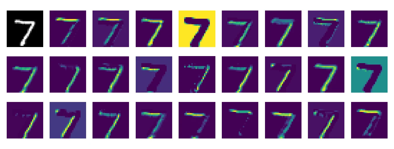

After one epoch the test accuracy is already 98.1 percent and after three it is 98.84 percent: 116 mistakes out of 10,000 digits. Notice the last batch loss jumping around (0.013 at epoch 2, 0.103 at epoch 3). That is mini-batch noise from Session 7, not a bug.
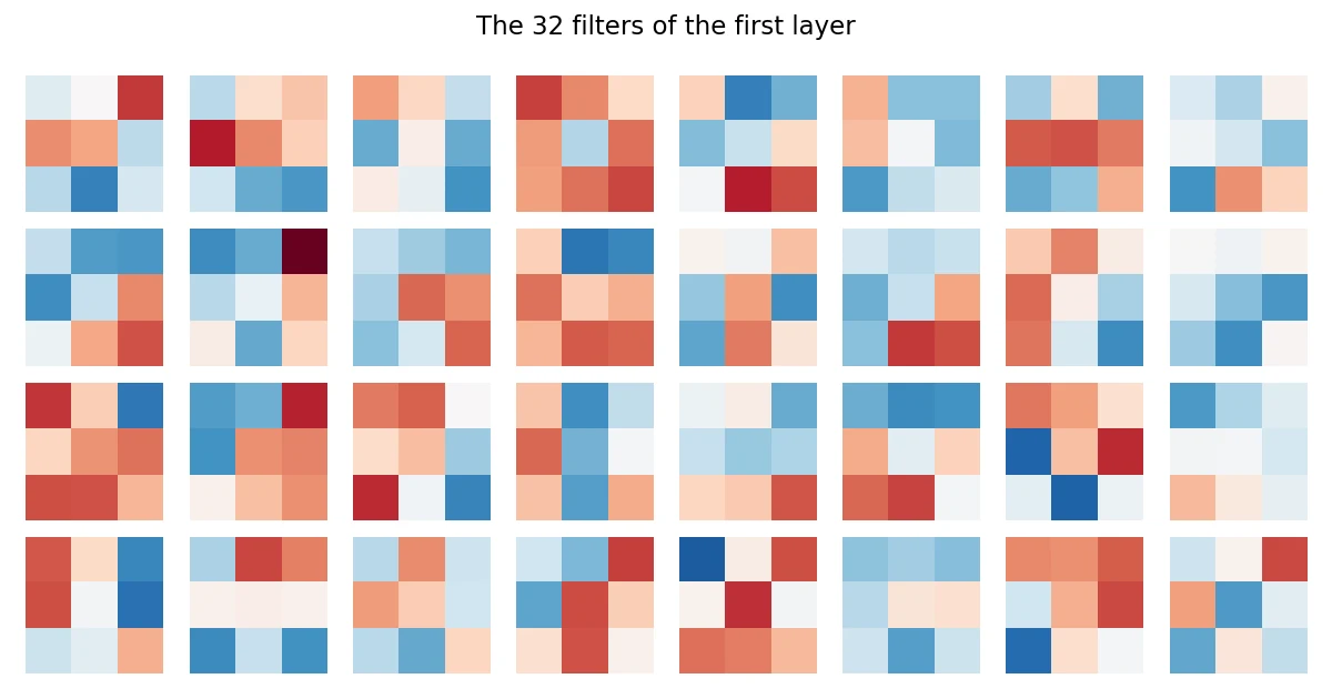
The first picture shows the 32 filters the first layer learned. Nobody drew them. Do not expect textbook-clean pictures after only three epochs on a small network: a few show a clear red-against-blue split, the signature of an edge detector, but most are untidy mixtures. That is normal, since the network only needs filters that work together, not ones a person can name. The second picture shows what the network "sees" in one digit, one feature map per filter. The third shows some of the 116 digits it still gets wrong, and many of them would make a person hesitate too.
The first widely successful CNN, LeNet, was built by Yann LeCun and colleagues in the 1990s to read handwritten digits on bank cheques. The network we trained is a direct descendant of that design.LeCun et al., 1998
A convolutional layer has 16 filters of size 3x3 and its input has 3 channels (an RGB image). How many parameters does it have?
CNN against a plain network
Is the convolution really worth it? Let us train a plain fully connected network (MLP) and a much smaller CNN for 2 epochs each, then test both on normal digits and on digits shifted 3 pixels down and right.
import torch
import torch.nn as nn
import torchvision
from torch.utils.data import DataLoader, TensorDataset

torch.manual_seed(0)
train = torchvision.datasets.MNIST("data", train=True, download=True)
test = torchvision.datasets.MNIST("data", train=False, download=True)
prep = lambda ds: ((ds.data.float() / 255 - 0.1307) / 0.3081).unsqueeze(1)
X_tr, y_tr, X_te, y_te = prep(train), train.targets, prep(test), test.targets
loader = DataLoader(TensorDataset(X_tr, y_tr), batch_size=128, shuffle=True)

mlp = nn.Sequential(nn.Flatten(), nn.Linear(784, 128), nn.ReLU(), nn.Linear(128, 10))
cnn = nn.Sequential(nn.Conv2d(1, 8, 3), nn.ReLU(), nn.MaxPool2d(2), nn.Conv2d(8, 16, 3), nn.ReLU(), nn.MaxPool2d(2),
                    nn.Flatten(), nn.Linear(16 * 5 * 5, 10))

def fit(model, epochs=2):
    opt = torch.optim.Adam(model.parameters(), lr=1e-3)
    for _ in range(epochs):
        model.train()
        for xb, yb in loader:
            loss = nn.functional.cross_entropy(model(xb), yb); opt.zero_grad(); loss.backward(); opt.step()
    return model.eval()

def acc(model, X):
    with torch.no_grad():
        return (model(X).argmax(1) == y_te).float().mean().item()

shifted = torch.roll(X_te, shifts=(3, 3), dims=(2, 3))          # slide every digit 3 pixels down and right
print("model   parameters   normal test   shifted test")
for name, m in [("MLP", fit(mlp)), ("CNN", fit(cnn))]:
print(f"{name} {sum(p.numel() for p in m.parameters()):8,d} {acc(m, X_te):.3f} {acc(m, shifted):.3f}")model parameters normal test shifted test
MLP 101,770 0.965 0.172
CNN 5,258 0.973 0.336The small CNN has 5,258 parameters, the MLP has 101,770, about 19 times more. And yet the CNN is already more accurate on normal digits (0.973 against 0.965). Then the shifted test: the MLP collapses to 0.172 and the CNN falls to 0.336. Two lessons, one reassuring and one honest. The CNN is far more robust to a shift, since its filters work wherever a stroke appears. But it is not magically shift-proof: pooling gives only a little tolerance, and the CNN was never shown shifted digits in training. That is why real systems use data augmentation (training on randomly shifted, rotated and flipped copies).
Where CNNs are used, and what they cost
CNNs read medical scans, power the camera on your phone, drive object detection (the next session), read licence plates and check manufactured parts for defects. They also work beyond pictures, wherever data has a grid structure, such as audio spectrograms.
| Strengths | Weaknesses |
|---|---|
| Learn their own features from raw pixels | Need a lot of labelled images |
| Far fewer parameters than a dense network | Expensive to train without a GPU |
| Reuse one filter everywhere (weight sharing) | Hard to interpret |
| Strong with augmentation and pre-trained weights | Expect a fixed-size grid and have no memory of order |
That last point is the wall of the CNN. It reads its input as a fixed grid and has no sense of "what came before", so it is the wrong tool for sentences, speech or price histories. That is Session 18. First, Session 17 shows how far the CNN idea can go.
import torch.nn as nn

cnn = nn.Sequential(
    nn.Conv2d(1, 32, kernel_size=3), nn.ReLU(), nn.MaxPool2d(2),
    nn.Conv2d(32, 64, kernel_size=3), nn.ReLU(), nn.MaxPool2d(2),
    nn.Flatten(),
    nn.Linear(64 * 5 * 5, 64), nn.ReLU(),
    nn.Linear(64, 10),                      # 10 digit classes (logits)
)
loss_fn = nn.CrossEntropyLoss() # applies softmax internallyWhy does a CNN need far fewer parameters than a fully connected network on the same image?
Try it yourself
- In
conv_by_hand.py, replace the kernel with[[1, 1, 1], [0, 0, 0], [-1, -1, -1]]. What kind of edge does it find? - Add
padding=1to the firstConv2dinshapes_and_params.pyand re-run. How does every later shape change? - Train
train_cnn.pyfor 1 epoch with only half the filters (16 and 32). How much accuracy do you lose? - In
mlp_vs_cnn.py, train the CNN on randomly shifted training images and test again on the shifted set.
What comes next
You can now explain how a network learns to see. Session 17 is an optional deep dive into the most popular application of the idea, object detection with YOLO, where the network does not just say what is in the picture but where. If you want to stay on the main road, Session 18 turns to sequences.
Frequently asked questions
What is a convolutional neural network in simple words?
A CNN is a neural network for grid-like data such as images. Instead of connecting every pixel to every neuron, it slides small learnable filters over the image to detect local patterns like edges, and stacks layers so that later ones detect shapes and objects.
What does a filter or kernel do in a CNN?
A filter is a small grid of learned weights, such as 3 by 3. It slides over the image, multiplying and summing at each position to produce a feature map showing where its pattern appears. A layer has many filters, each learning a different pattern.
What is the purpose of pooling?
Pooling shrinks the feature maps, which reduces computation and the number of parameters, and gives the network a little tolerance to small shifts. Max pooling keeps the largest value in each window.
What are stride and padding?
Stride is how many pixels the filter moves at each step, and larger strides give smaller outputs. Padding adds a border of zeros around the image so the output keeps its size and border pixels are not under-used.
Why do CNNs work better than ordinary neural networks on images?
They exploit the structure of images: patterns are local and the same pattern can appear anywhere. Local filters with shared weights need far fewer parameters and generalise better than dense layers that treat every pixel independently.