
In Session 2 a straight line worked until it did not. Two problems showed up. When two features carried almost the same information, the weights went wild: s1 at -931 and s2 at +518, cancelling each other out. And a very flexible curve threatened to chase noise instead of signal.
Both problems have the same family of fixes, called regularization. The idea is simple enough to say in one sentence. Make the model pay a price for having big weights, and it will only keep the weights it really needs. This session shows how that works, why two flavours (Ridge and Lasso) behave differently, and when to use which.
Overfitting and underfitting: the two ways to fail
Picture two students before an exam. One barely studied, so they get everything wrong. The other memorised last year's paper word for word, so they do brilliantly on the practice questions and collapse on anything new. Models fail in exactly these two ways.
- Underfitting. The model is too simple to capture the pattern. It does badly on the training data and on new data. People call this high bias.
- Overfitting. The model is so flexible that it memorises the training data, noise included. It does brilliantly on training data and badly on new data. People call this high variance.
The code below makes it visible. Same noisy data, three models of rising flexibility (a polynomial of degree 1, 4 and 14). Half the points train the model, half are held back to test it.
import numpy as np
import matplotlib.pyplot as plt
from sklearn.linear_model import LinearRegression
from sklearn.metrics import r2_score
from sklearn.pipeline import make_pipeline
from sklearn.preprocessing import PolynomialFeatures, StandardScaler

rng = np.random.default_rng(0)
x = np.sort(rng.uniform(0, 1, 30))
y = np.sin(2 * np.pi * x) + rng.normal(0, 0.25, 30)       # a smooth signal plus noise
x_tr, y_tr = x[::2], y[::2]                               # 15 points to learn from
x_te, y_te = x[1::2], y[1::2]                             # 15 points held back

grid = np.linspace(0, 1, 200)
fig, ax = plt.subplots(1, 3, figsize=(11, 3.4), sharey=True)
for a, degree in zip(ax, [1, 4, 14]):
    m = make_pipeline(PolynomialFeatures(degree), StandardScaler(), LinearRegression())
    m.fit(x_tr.reshape(-1, 1), y_tr)
    tr = r2_score(y_tr, m.predict(x_tr.reshape(-1, 1)))
    te = r2_score(y_te, m.predict(x_te.reshape(-1, 1)))
    print(f"degree {degree:2d}   train R² {tr:6.3f}   test R² {te:8.3f}")
    a.scatter(x_tr, y_tr, s=22, color="#2563EB", label="train")
    a.scatter(x_te, y_te, s=22, color="#F59E0B", label="test")
    a.plot(grid, np.clip(m.predict(grid.reshape(-1, 1)), -2.5, 2.5), color="#DC2626", lw=2)
    a.set_title(f"degree {degree}"); a.set_ylim(-2.5, 2.5)
    a.spines[["top", "right"]].set_visible(False)
ax[0].legend(frameon=False, loc="lower left")
fig.tight_layout()degree 1 train R² 0.461 test R² 0.392
degree 4 train R² 0.909 test R² 0.864
degree 14 train R² 1.000 test R² -49.580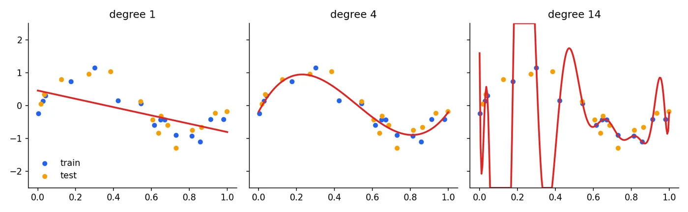
Read the three lines of output first. Degree 1 is too stiff: R² of 0.46 on training data and 0.39 on test data, both poor, so it is underfitting. Degree 4 is about right: 0.91 and 0.86, close to each other and both good. Degree 14 has a perfect training score of 1.000 and a test score of -49.6. That is not a typo. A negative R² means the model is worse than just predicting the average, and here it is catastrophically worse, because the curve swings wildly between the training points.
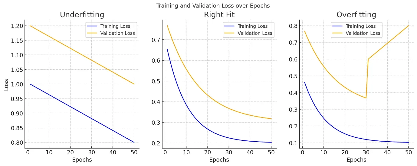
The warning sign is the gap. A big gap between training and test scores means overfitting. Two low scores that are close together means underfitting.
The expected squared error of a model splits into three parts. Bias is the error from assumptions that are too simple. Variance is the error from reacting too much to the particular training sample. is noise nobody can remove. Making a model more flexible lowers bias and raises variance, so we are looking for the sweet spot. Session 13 returns to this when we meet bagging and boosting.
What regularization does
A model that overfits usually does so by giving some features huge weights that twist the curve to hit individual training points. Regularization attacks that directly. We keep the normal loss (how wrong the predictions are) and add a penalty that grows with the size of the weights:
("lambda") sets how much we care about the penalty. gives back plain least squares. A huge forces every weight towards zero and the model becomes useless. In scikit-learn this knob is called alpha. is the penalty, and its shape is what separates Ridge from Lasso.
Now the model has a trade-off. Large weights reduce the first term and increase the second. The best weights are the smallest ones that still explain the data well.
Ridge regression (L2)
Ridge adds the sum of the squared weights:
is the number of features. Squaring means one very large weight is punished far more than several small ones, so Ridge spreads the weight across correlated features instead of piling it onto one. It shrinks weights smoothly towards zero but never exactly to zero. The intercept is not penalised.
Ridge even has a tidy closed-form answer, a small tweak of the normal equation from Session 2. The term also makes the matrix easier to invert, which is why Ridge stays stable when features are nearly copies of each other:
is the identity matrix (ones on the diagonal, zeros elsewhere). This formula assumes the features and target are centred, which is what a scaling step gives you.
Lasso regression (L1)
Lasso adds the sum of the absolute values of the weights instead:
Lasso stands for Least Absolute Shrinkage and Selection Operator. The absolute value has a sharp corner at zero, and that corner is exactly why Lasso can push weights to exactly zero. A weight at zero means that feature is out of the model, so Lasso also performs feature selection.
The scikit-learn objectives are scaled a little differently. Ridge minimises ||y - Xw||² + alpha * ||w||², while Lasso minimises (1 / (2 * n_samples)) * ||y - Xw||² + alpha * ||w||₁. So the same alpha number does not mean the same penalty strength in the two models. Pick alpha separately for each, ideally by cross-validation (below).
Why Lasso gives zeros and Ridge does not
Here is the picture behind it. Each pair of weights has some error. The blue rings are lines of equal error, lowest at the centre, which is where plain least squares would land. The penalty says "stay inside this orange region". The answer is the point where the rings first touch the region.
import numpy as np
import matplotlib.pyplot as plt

fig, ax = plt.subplots(1, 2, figsize=(9, 4.2))
t = np.linspace(0, 2 * np.pi, 400)
gx, gy = np.meshgrid(np.linspace(-2.2, 2.2, 300), np.linspace(-2.2, 2.2, 300))
# the error surface: ellipses centred on the unpenalised best weights (1.6, 0.5)
err = (gx - 1.6) ** 2 * 1.0 + (gy - 0.5) ** 2 * 3.0 + 0.8 * (gx - 1.6) * (gy - 0.5)
for a, kind in zip(ax, ["L1 (Lasso): a diamond", "L2 (Ridge): a circle"]):
    a.contour(gx, gy, err, levels=[0.3, 0.8, 1.6, 2.6], colors="#2563EB", linewidths=1.2)
    if kind.startswith("L1"):
        a.fill([1.0, 0, -1.0, 0], [0, 1.0, 0, -1.0], color="#F59E0B", alpha=.35)
        a.plot([1.0, 0, -1.0, 0, 1.0], [0, 1.0, 0, -1.0, 0], color="#D97706", lw=2)
        a.scatter([1.0], [0], color="#DC2626", zorder=5)
        a.annotate("solution lands on a corner:\nw2 is exactly 0", (1.0, 0), (0.15, -1.75), fontsize=9, arrowprops=dict(arrowstyle="->"))
    else:
        a.fill(np.cos(t), np.sin(t), color="#F59E0B", alpha=.35)
        a.plot(np.cos(t), np.sin(t), color="#D97706", lw=2)
        a.scatter([0.96], [0.28], color="#DC2626", zorder=5)
        a.annotate("solution slides along the\nsmooth edge: both weights\nsmall, neither zero", (0.96, 0.28), (-2.1, -1.75), fontsize=9, arrowprops=dict(arrowstyle="->"))
    a.axhline(0, color="#9CA3AF", lw=.8); a.axvline(0, color="#9CA3AF", lw=.8)
    a.set_title(kind); a.set_xlabel("weight w1"); a.set_ylabel("weight w2"); a.set_aspect("equal")
    a.spines[["top", "right"]].set_visible(False)
fig.tight_layout()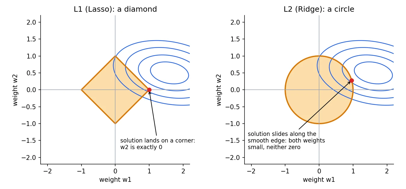
The L1 region is a diamond, and a diamond has sharp corners that sit on the axes. The rings are very likely to touch a corner first, and at a corner one weight is exactly zero. The L2 region is a smooth circle with no corners, so the rings touch it somewhere along the edge, where both weights are small but non-zero.
Ridge regression was introduced by Arthur Hoerl and Robert Kennard in 1970. Lasso came much later, from Stanford's Robert Tibshirani, in 1996.Technometrics 1970; Journal of the Royal Statistical Society B, 1996
See it on real data
Same diabetes dataset and the same train/test split as before. Two rules for regularized models, both enforced in the code: scale the features first (otherwise the penalty punishes a feature just because its units are large) and keep the scaler inside a pipeline (Session 1's leakage lesson).
import numpy as np
import pandas as pd
from sklearn.datasets import load_diabetes
from sklearn.linear_model import LinearRegression, Ridge, Lasso, ElasticNet
from sklearn.metrics import r2_score
from sklearn.model_selection import train_test_split
from sklearn.pipeline import make_pipeline
from sklearn.preprocessing import StandardScaler

data = load_diabetes(as_frame=True)
X, y = data.data, data.target
X_tr, X_te, y_tr, y_te = train_test_split(X, y, test_size=0.2, random_state=42)

models = {
    "OLS (no penalty)": LinearRegression(),
    "Ridge  alpha=10":   Ridge(alpha=10),
    "Lasso  alpha=2":    Lasso(alpha=2),
    "ElasticNet":        ElasticNet(alpha=1, l1_ratio=0.5),
}
rows, coefs = [], {}
for name, est in models.items():
    pipe = make_pipeline(StandardScaler(), est).fit(X_tr, y_tr)   # scale first, always
    rows.append((name, r2_score(y_tr, pipe.predict(X_tr)), r2_score(y_te, pipe.predict(X_te))))
    coefs[name.split()[0]] = pipe[-1].coef_

print(pd.DataFrame(rows, columns=["model", "train R²", "test R²"]).round(3).to_string(index=False))
print()
print((pd.DataFrame(coefs, index=X.columns).round(1) + 0.0).to_string())   # + 0.0 turns -0.0 into 0.0
print("\nfeatures Lasso set to exactly zero:", [c for c, w in zip(X.columns, coefs["Lasso"]) if w == 0]) model train R² test R²
OLS (no penalty) 0.528 0.453
Ridge alpha=10 0.525 0.457
Lasso alpha=2 0.517 0.472
ElasticNet 0.493 0.455
OLS Ridge Lasso ElasticNet
age 1.8 1.9 0.0 1.8
sex -11.5 -11.0 -7.4 -6.0
bmi 25.6 25.6 26.1 19.0
bp 16.8 16.3 14.7 12.3
s1 -44.4 -12.9 -4.1 -1.2
s2 24.6 0.5 0.0 -2.9
s3 7.7 -6.1 -10.9 -8.4
s4 13.1 8.6 0.0 5.8
s5 35.2 22.7 21.5 14.4
s6 2.4 2.9 1.5 5.0
features Lasso set to exactly zero: ['age', 's2', 's4']Let's read it properly.
The scores. All four models land in the same neighbourhood on test data (0.45 to 0.47). Regularization did not suddenly produce a miracle here, and that is honest: the diabetes data has only ten features and 353 training rows, so plain regression was never badly overfitted. Lasso is a little better, 0.472 against 0.453, and it needs fewer features to get there.
The weights, and the Session 2 mystery solved. Look at s1 and s2. Plain regression has -44.4 and +24.6, huge and opposite (these are weights per standardised unit, so the numbers differ from Session 2's raw ones, but the pattern is the same). Ridge pulls them to -12.9 and +0.5. Lasso goes further and sets s2 to exactly zero, keeping a small s1. The wild cancelling pair is gone. Lasso also removed age and s4, which carry little extra information.
That is the real payoff of regularization: not always a higher score, but weights you can trust and a simpler model that holds up on new data.
Watching the penalty at work
How does the result change as the penalty grows? Plot every weight against alpha:
import numpy as np
import matplotlib.pyplot as plt
from sklearn.datasets import load_diabetes
from sklearn.linear_model import Ridge, Lasso
from sklearn.preprocessing import StandardScaler

data = load_diabetes()
X = StandardScaler().fit_transform(data.data)
y = data.target
alphas = np.logspace(-2, 3, 60)

fig, ax = plt.subplots(1, 2, figsize=(10.5, 3.8), sharey=True)
for a, Model, title in [(ax[0], Ridge, "Ridge (L2): weights shrink smoothly"), (ax[1], Lasso, "Lasso (L1): weights hit exactly zero")]:
    W = np.array([Model(alpha=al, max_iter=20000).fit(X, y).coef_ for al in alphas])
    for j, name in enumerate(data.feature_names):
        a.plot(alphas, W[:, j], lw=1.8, label=name)
    a.set_xscale("log"); a.set_xlabel("alpha (penalty strength)"); a.set_title(title)
    a.axhline(0, color="#9CA3AF", lw=.8); a.spines[["top", "right"]].set_visible(False)
ax[0].set_ylabel("weight")
ax[1].legend(ncol=2, fontsize=8, frameon=False, loc="upper right")
fig.tight_layout()
print("Lasso at alpha=10 keeps", int((Lasso(alpha=10).fit(X, y).coef_ != 0).sum()), "of 10 features")Lasso at alpha=10 keeps 4 of 10 features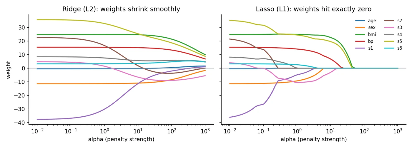
On the left, Ridge: every curve glides smoothly towards zero as alpha grows, none touching it. On the right, Lasso: the weights drop out one at a time, the least useful ones first, and stay at zero. At alpha = 10, Lasso keeps just four of the ten features. If you wanted to know which features matter most, the order in which they die is a good clue.
Which regularization method can set some feature weights to exactly zero, removing those features?
Choosing the penalty strength
alpha is a hyperparameter: a setting we choose, not one the model learns. Too small and you are back to overfitting. Too large and you underfit. The standard way to choose is cross-validation: split the training data into 5 parts, train on 4, validate on 1, rotate, and average. scikit-learn has this built in as RidgeCV and LassoCV.
import numpy as np
from sklearn.datasets import load_diabetes
from sklearn.linear_model import LassoCV, RidgeCV
from sklearn.metrics import r2_score
from sklearn.model_selection import train_test_split
from sklearn.pipeline import make_pipeline
from sklearn.preprocessing import StandardScaler

X, y = load_diabetes(return_X_y=True)
X_tr, X_te, y_tr, y_te = train_test_split(X, y, test_size=0.2, random_state=42)

ridge = make_pipeline(StandardScaler(), RidgeCV(alphas=np.logspace(-2, 3, 40), cv=5)).fit(X_tr, y_tr)
lasso = make_pipeline(StandardScaler(), LassoCV(alphas=np.logspace(-3, 1, 40), cv=5, max_iter=20000)).fit(X_tr, y_tr)

print("Ridge picked alpha =", round(ridge[-1].alpha_, 2), "| test R² =", round(r2_score(y_te, ridge.predict(X_te)), 3))
print("Lasso picked alpha =", round(lasso[-1].alpha_, 2), "| test R² =", round(r2_score(y_te, lasso.predict(X_te)), 3))
print("Lasso kept", int((lasso[-1].coef_ != 0).sum()), "of 10 features")Ridge picked alpha = 38.88 | test R² = 0.46
Lasso picked alpha = 1.51 | test R² = 0.471
Lasso kept 8 of 10 featuresNotice the pattern: it tried 40 values of alpha, judged them only on validation folds inside the training data, and the test set was touched once at the very end. We go much deeper on tuning in Session 5.
Ridge, Lasso or ElasticNet?
| Situation | Reach for | Why |
|---|---|---|
| Many features, you suspect most are useless | Lasso | Drops the useless ones, gives a sparse model |
| Features strongly correlated with each other | Ridge | Spreads weight evenly and keeps all features stable |
| Many correlated features and you also want selection | ElasticNet | Mixes both penalties with l1_ratio |
| Few features, plenty of data | Plain regression, or tiny alpha |
Little to gain from a penalty |
A caution about Lasso: when a group of features is highly correlated, it tends to pick one of them more or less arbitrarily and drop the rest. If that matters to you, ElasticNet is the safer choice.
("rho") is l1_ratio in scikit-learn. is pure Lasso and is pure Ridge, with every blend in between.
from sklearn.linear_model import Ridge, Lasso, ElasticNet
from sklearn.pipeline import make_pipeline
from sklearn.preprocessing import StandardScaler

ridge = make_pipeline(StandardScaler(), Ridge(alpha=1.0)).fit(X_train, y_train)
lasso = make_pipeline(StandardScaler(), Lasso(alpha=0.1)).fit(X_train, y_train)
enet  = make_pipeline(StandardScaler(), ElasticNet(alpha=0.1, l1_ratio=0.5)).fit(X_train, y_train)

print(lasso[-1].coef_)     # zeros mean Lasso dropped those features
Regularization is not only for regression. Weight decay in neural networks is the same L2 idea, and it is one of the settings used when training today's large language models.
Other ways to regularize
The penalty is only one tool. You will meet others as the course goes on:
- Dropout: randomly switching off neurons during training (neural networks, Session 9).
- Early stopping: halting training when validation loss starts to rise (Session 5).
- Data augmentation: feeding more varied versions of your existing data, such as flipped or cropped images.
- A simpler model: fewer layers, fewer neurons, shallower trees.
- More data: the most reliable cure of all, when you can get it.
Why must you scale features before applying Ridge or Lasso?
Try it yourself
- Change the
alphaof the Ridge model in the code to 0.01, then 1000. What happens to the train and test R²? Which direction is underfitting? - In
overfit_polynomial.py, addRidge(alpha=1)in place ofLinearRegression()for the degree 14 model. Can a penalty rescue a model that flexible? - Run Lasso with
alpha=5, and list which features survive. Does the set match the order they disappear in the regularization-path figure? - Try ElasticNet with
l1_ratioof 0.1, 0.5 and 0.9, and watch how the number of zero weights changes.
What comes next
We have been judging models with a single number, R², and glossing over what it hides. In Session 4 we look at how to measure models properly: MAE, MSE and R² for numbers, and the confusion matrix, precision, recall and F1 for categories.
Frequently asked questions
What is the difference between L1 and L2 regularization?
L1 (Lasso) adds the sum of absolute weights as a penalty and can shrink some weights exactly to zero, which removes features. L2 (Ridge) adds the sum of squared weights and shrinks all weights smoothly towards zero without removing any. L1 gives sparse models, L2 gives stable ones.
When should I use Ridge instead of Lasso?
Use Ridge when you have many features that are correlated with each other and you want to keep them all while stabilising the weights. Use Lasso when you suspect many features are useless and you want the model to drop them.
What does the alpha (lambda) parameter control?
It sets the strength of the penalty. Zero is plain least squares, a small value gives a gentle penalty and a large value shrinks weights hard. Because it is a hyperparameter, choose it with cross-validation, for example RidgeCV or LassoCV.
How do I know if my model is overfitting?
Compare training and test performance. A model that scores very well on training data and much worse on test data is overfitting. If both scores are low and close together, it is underfitting. Plotting training and validation loss over time shows the same thing.
Does regularization always improve the test score?
No. It helps most when the model is flexible relative to the amount of data, or when features are correlated. On a small, clean problem it may change the score very little, as in our diabetes example, though it still makes the weights more trustworthy.