
Neural networks are powerful, but ask one why it made a decision and you mostly get a shrug. A decision tree is the opposite. It is a flowchart of yes/no questions that a person can read, check and explain to a bank manager or a doctor. For spreadsheets of rows and columns, trees and their descendants are still some of the best models in the world.
Part III takes the second road to non-linearity from the course story: instead of stacking neurons, we split the data with simple questions. This session is the foundation for everything in the part. We will see how a tree decides which question to ask, work through the numbers by hand on a classic example, and watch a single tree overfit. It leans on overfitting from Session 3 and the metrics of Session 4.
What a decision tree is
A tree is built from a few parts:
- The root node is the first question, where the whole dataset starts.
- Decision nodes are the questions further down.
- Leaf nodes (terminal nodes) hold the final answer. No more questions are asked.
- A branch is one path of answers, and a sub-tree is a section of the whole.
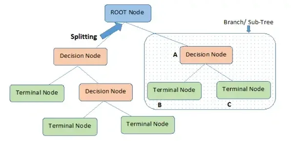
The same structure predicts categories (classification trees) and numbers (regression trees). It is called non-parametric because it does not have a fixed number of weights set in advance. A neural network's size is decided before training. A tree grows as the data grows: more data allows more splits and a more flexible model.
| Parametric (linear models, neural nets) | Non-parametric (trees, KNN) | |
|---|---|---|
| Structure | Fixed beforehand | Grows with the data |
| Complexity | Stays the same as data grows | Increases with more data |
| Assumptions | Assumes a shape (for example linear) | Assumes none |
Trees also have practical perks: they need no feature scaling, they handle mixed numeric and categorical data once encoded, and they mimic how people reason.
How a tree picks a question
Think of the game 20 Questions. A good first question splits the possibilities into clean halves, a bad one wastes a turn. A tree plays that game with your data. At every node it tries every possible question ("is income above 100k?", "is humidity high?") and keeps the one that makes the resulting groups purest, meaning as dominated by one class as possible.
So we need a number for "how mixed is this group?". There are two standard ones.
is the share of class in the node and is the number of classes. A pure node (all one class) has . For two classes, a 50/50 mix has the maximum . It is the default in scikit-learn.
Borrowed from information theory (the same Shannon idea behind cross-entropy in Session 6). A pure node has , and a 50/50 two-class mix has the maximum bit.
import numpy as np
import matplotlib.pyplot as plt

p = np.linspace(0.001, 0.999, 400)
gini = 1 - p ** 2 - (1 - p) ** 2
entropy = -(p * np.log2(p) + (1 - p) * np.log2(1 - p))

fig, ax = plt.subplots(figsize=(6.2, 3.6))
ax.plot(p, entropy, lw=2.2, color="#7C3AED", label="entropy")
ax.plot(p, gini, lw=2.2, color="#0D9488", label="Gini impurity")
ax.set_xlabel("share of class 1 in the node"); ax.set_ylabel("impurity")
ax.legend(frameon=False); ax.spines[["top", "right"]].set_visible(False)
fig.tight_layout()

for share in (1.0, 0.9, 0.5):
    g = 1 - share ** 2 - (1 - share) ** 2
    e = 0.0 if share in (0, 1) else -(share * np.log2(share) + (1 - share) * np.log2(1 - share))
print(f"node with {share:.0%} class 1: Gini {g:.3f} entropy {e:.3f}")node with 100% class 1: Gini 0.000 entropy 0.000
node with 90% class 1: Gini 0.180 entropy 0.469
node with 50% class 1: Gini 0.500 entropy 1.000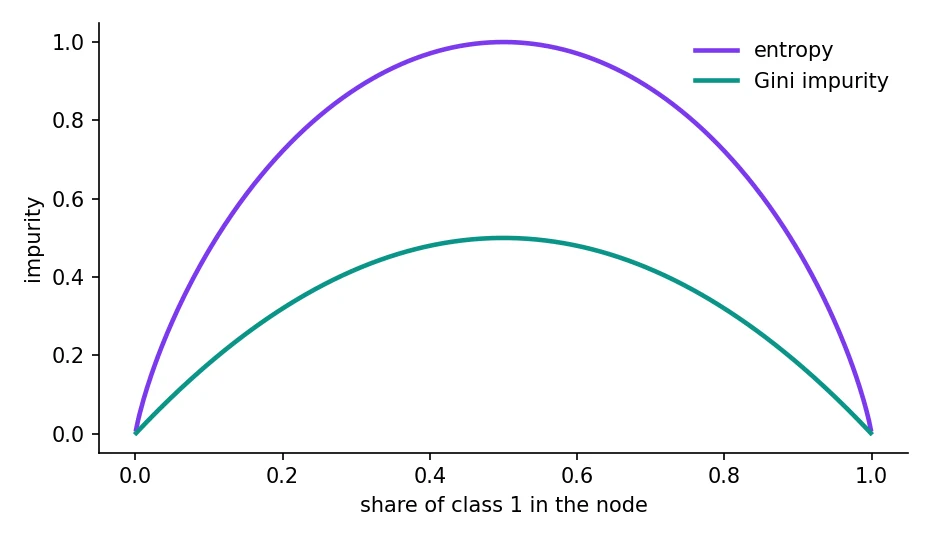
Both fall to zero for a pure node and peak at a 50/50 mix, and in practice they choose almost the same splits. Gini is a little cheaper to compute because it has no logarithm.
To choose a split, the tree compares the impurity before with the weighted average impurity of the two groups after. That drop is the information gain (when entropy is used) or the impurity decrease (for Gini):
is the number of rows in the parent node and the number in child . Each child's entropy is weighted by how many rows it holds, so a tiny pure child cannot fake a good split. The tree picks the question with the highest gain.
A worked example: should we play tennis?
This is the classic teaching dataset: 14 days, four weather facts, and whether tennis was played. Nine days were "Yes" and five "No". Below we compute the entropy of the whole table and then the information gain of every possible first question, exactly the way a tree does it.
import numpy as np
import pandas as pd
from sklearn.tree import DecisionTreeClassifier, export_text

# The classic 14-day "should we play tennis?" table
rows = [
 ("Sunny","Hot","High","Weak","No"),("Sunny","Hot","High","Strong","No"),("Overcast","Hot","High","Weak","Yes"),
 ("Rain","Mild","High","Weak","Yes"),("Rain","Cool","Normal","Weak","Yes"),("Rain","Cool","Normal","Strong","No"),
 ("Overcast","Cool","Normal","Strong","Yes"),("Sunny","Mild","High","Weak","No"),("Sunny","Cool","Normal","Weak","Yes"),
 ("Rain","Mild","Normal","Weak","Yes"),("Sunny","Mild","Normal","Strong","Yes"),("Overcast","Mild","High","Strong","Yes"),
 ("Overcast","Hot","Normal","Weak","Yes"),("Rain","Mild","High","Strong","No")]
df = pd.DataFrame(rows, columns=["outlook", "temp", "humidity", "wind", "play"])

def entropy(s):
    p = s.value_counts(normalize=True)
    return float(-(p * np.log2(p)).sum())

def gini(s):
    p = s.value_counts(normalize=True)
    return float(1 - (p ** 2).sum())

print(f"whole table: {df.play.value_counts().to_dict()}   entropy {entropy(df.play):.3f}   gini {gini(df.play):.3f}\n")
print("information gain of each possible first question:")
for col in ["outlook", "temp", "humidity", "wind"]:
    after = sum(len(g) / len(df) * entropy(g.play) for _, g in df.groupby(col))
    print(f"  {col:9s} gain = {entropy(df.play) - after:.3f}")

X = pd.get_dummies(df.drop(columns="play"))
tree = DecisionTreeClassifier(criterion="entropy", random_state=0).fit(X, df.play)
print("\nthe tree scikit-learn grows:")
print(export_text(tree, feature_names=list(X.columns)))whole table: {'Yes': 9, 'No': 5} entropy 0.940 gini 0.459
information gain of each possible first question:
outlook gain = 0.247
temp gain = 0.029
humidity gain = 0.152
wind gain = 0.048
the tree scikit-learn grows:
|--- outlook_Overcast <= 0.50
| |--- humidity_Normal <= 0.50
| | |--- outlook_Rain <= 0.50
| | | |--- class: No
| | |--- outlook_Rain > 0.50
| | | |--- wind_Strong <= 0.50
| | | | |--- class: Yes
| | | |--- wind_Strong > 0.50
| | | | |--- class: No
| |--- humidity_Normal > 0.50
| | |--- wind_Weak <= 0.50
| | | |--- temp_Cool <= 0.50
| | | | |--- class: Yes
| | | |--- temp_Cool > 0.50
| | | | |--- class: No
| | |--- wind_Weak > 0.50
| | | |--- class: Yes
|--- outlook_Overcast > 0.50
| |--- class: YesThe whole table has entropy 0.940 (a fairly mixed 9 to 5). Asking about the outlook gives a gain of 0.247, much higher than humidity (0.152), wind (0.048) or temperature (0.029). So the tree puts "outlook" at the root. That is not a coincidence: when the outlook is overcast, every single row is "Yes", a perfectly pure leaf right away. Sunny and rainy days are still mixed, so the tree asks a second question for each.
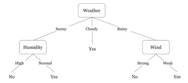
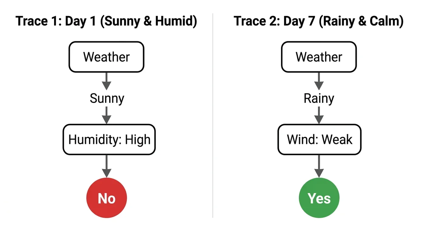
One detail from the output: scikit-learn grew a slightly different-looking tree. Its trees only make binary splits, so "outlook" with three values becomes a question like "is it overcast, yes or no?", and the rest is handled further down. The logic is the same, the shape differs.
For a feature and threshold , the tree computes this weighted impurity of the two groups and keeps the pair with the smallest value. That is the CART algorithm (Classification And Regression Trees), which scikit-learn uses. Numeric features are tested at thresholds between sorted values.
The two names behind most trees: CART was published in 1984 by Breiman, Friedman, Olshen and Stone, and Ross Quinlan's ID3 followed in 1986 (and C4.5 in 1993).Breiman et al., 1984; Quinlan, 1986
A node contains 10 rows, all of the same class. What are its Gini impurity and entropy?
Seeing a real tree
Now a bigger dataset: the breast-cancer data from Session 4, 569 tumours and 30 measurements. We limit the tree to depth 3 and at least 5 rows per leaf so that it stays readable.
import matplotlib.pyplot as plt
from sklearn.datasets import load_breast_cancer
from sklearn.model_selection import train_test_split
from sklearn.tree import DecisionTreeClassifier, plot_tree, export_text

data = load_breast_cancer()
X_tr, X_te, y_tr, y_te = train_test_split(data.data, data.target, test_size=0.3, random_state=3, stratify=data.target)

tree = DecisionTreeClassifier(criterion="gini", max_depth=3, min_samples_leaf=5, random_state=0).fit(X_tr, y_tr)
print("test accuracy:", round(tree.score(X_te, y_te), 3))
print(export_text(tree, feature_names=list(data.feature_names)))

fig, ax = plt.subplots(figsize=(11, 5))
plot_tree(tree, feature_names=data.feature_names, class_names=data.target_names, filled=True, rounded=True, fontsize=8, ax=ax)
fig.tight_layout()test accuracy: 0.942
|--- worst perimeter <= 106.10
| |--- worst concave points <= 0.14
| | |--- radius error <= 0.60
| | | |--- class: 1
| | |--- radius error > 0.60
| | | |--- class: 1
| |--- worst concave points > 0.14
| | |--- mean smoothness <= 0.11
| | | |--- class: 1
| | |--- mean smoothness > 0.11
| | | |--- class: 0
|--- worst perimeter > 106.10
| |--- worst texture <= 20.65
| | |--- worst perimeter <= 114.25
| | | |--- class: 1
| | |--- worst perimeter > 114.25
| | | |--- class: 0
| |--- worst texture > 20.65
| | |--- worst smoothness <= 0.11
| | | |--- class: 0
| | |--- worst smoothness > 0.11
| | | |--- class: 0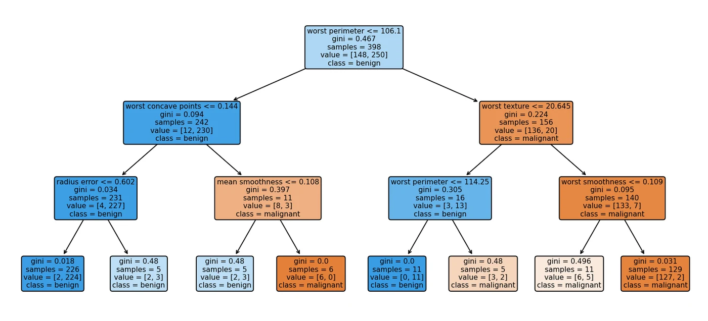
You can read the printout as plain English. "If the worst perimeter is 106.1 or less, and the worst concave points are 0.14 or less, predict class 1 (benign)." It scores 94.2 percent on unseen tumours using at most three short questions per tumour. This is why trees are loved in lending, healthcare and any field where a decision must be justified.
Where a single tree goes wrong
A tree that is allowed to keep splitting will keep going until every leaf is pure, which means it has memorised the training data, noise and all. That is overfitting with a new face. Watch the depth:
import matplotlib.pyplot as plt
from sklearn.datasets import load_breast_cancer
from sklearn.model_selection import train_test_split
from sklearn.tree import DecisionTreeClassifier

X, y = load_breast_cancer(return_X_y=True)
X_tr, X_te, y_tr, y_te = train_test_split(X, y, test_size=0.3, random_state=3, stratify=y)

depths = range(1, 13)
train_acc, test_acc = [], []
for d in depths:
    t = DecisionTreeClassifier(max_depth=d, random_state=0).fit(X_tr, y_tr)
    train_acc.append(t.score(X_tr, y_tr)); test_acc.append(t.score(X_te, y_te))
    if d in (1, 2, 3, 5, 12):
        print(f"max_depth {d:2d}   leaves {t.get_n_leaves():3d}   train {train_acc[-1]:.3f}   test {test_acc[-1]:.3f}")

fig, ax = plt.subplots(figsize=(6.4, 3.7))
ax.plot(list(depths), train_acc, "-o", ms=4, lw=2, color="#2563EB", label="train")
ax.plot(list(depths), test_acc, "-o", ms=4, lw=2, color="#F59E0B", label="test")
ax.set_xlabel("max_depth"); ax.set_ylabel("accuracy"); ax.legend(frameon=False); ax.spines[["top", "right"]].set_visible(False)
fig.tight_layout()max_depth 1 leaves 2 train 0.920 test 0.918
max_depth 2 leaves 4 train 0.957 test 0.895
max_depth 3 leaves 8 train 0.975 test 0.924
max_depth 5 leaves 15 train 0.997 test 0.930
max_depth 12 leaves 16 train 1.000 test 0.906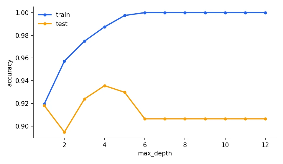
Training accuracy climbs steadily and reaches 1.000 at the deepest setting. Test accuracy tells another story: 0.918 at depth 1, a wobble down to 0.895 at depth 2, a peak of 0.930 at depth 5 and then a fall to 0.906 at depth 12. The extra depth after about 5 buys nothing on new data. (The data set is small, so test accuracy is noisy, which is itself part of the lesson.)
There is a second weakness, and it is the one the next session fixes. Trees are unstable: change the data a little and you can get a completely different tree.
import numpy as np
from sklearn.datasets import load_breast_cancer
from sklearn.tree import DecisionTreeClassifier

data = load_breast_cancer()
X, y = data.data, data.target
rng = np.random.default_rng(0)

print("five trees, each trained on a random 80% of the same data:")
for i in range(5):
    idx = rng.choice(len(X), size=int(0.8 * len(X)), replace=False)
    t = DecisionTreeClassifier(random_state=0).fit(X[idx], y[idx])
    root = data.feature_names[t.tree_.feature[0]]
print(f" tree {i + 1}: root question = '{root} <= {t.tree_.threshold[0]:.3f}' leaves = {t.get_n_leaves()}")five trees, each trained on a random 80% of the same data:
tree 1: root question = 'worst area <= 868.200' leaves = 19
tree 2: root question = 'worst concave points <= 0.145' leaves = 21
tree 3: root question = 'worst radius <= 16.795' leaves = 16
tree 4: root question = 'worst radius <= 16.795' leaves = 20
tree 5: root question = 'worst radius <= 16.795' leaves = 16Five trees, each trained on a random 80 percent of the same patients. Three different questions were chosen for the root (worst area, worst concave points and worst radius), and the number of leaves ranged from 16 to 21. A model that changes this much with a small change in the data has high variance.
Controlling growth: pruning
The remedy is to stop the tree growing too wild, which is called pruning. Two flavours:
- Pre-pruning: set limits before training, such as
max_depth,min_samples_leaf(the minimum rows a leaf must hold) ormin_samples_split. - Post-pruning: grow a big tree, then cut back branches that do not help. In scikit-learn this is cost-complexity pruning, controlled by
ccp_alpha.
is the tree's error on the training data, the number of leaves and a penalty per leaf. It is the same idea as Ridge and Lasso in Session 3: pay a price for complexity. Larger means a smaller tree.
from sklearn.tree import DecisionTreeClassifier, plot_tree

tree = DecisionTreeClassifier(criterion="gini", max_depth=3, min_samples_leaf=5, random_state=0)
tree.fit(X_train, y_train)
print(tree.score(X_test, y_test))
plot_tree(tree, feature_names=feature_names, class_names=class_names, filled=True)A regression tree splits the same way but predicts the average of the training rows in each leaf, and it chooses splits that minimise the mean squared error instead of Gini. Its predictions look like a staircase, and, like a classification tree, a very deep one overfits.
Why is a very deep decision tree usually a bad idea?
Try it yourself
- In
tennis_tree.py, change one row, for example make Day 4 a "No". Do the information gains change? Does the root question change? - In
depth.py, addmin_samples_leaf=10to the tree. Does the training-versus-test gap close? - Re-run
instability.pywithrandom_statevalues 1 and 2. How often does the root question change? - Fit
DecisionTreeRegressoron the diabetes data from Part I and compare its test R² with the linear regression's 0.453.
What comes next
A single tree is easy to understand and easy to overfit, and it changes a lot when the data shifts slightly. The classical fix is to stop trusting one tree and let hundreds of them vote. Session 12 builds that forest.
Frequently asked questions
What is the difference between Gini impurity and entropy?
Both measure how mixed a node is, with 0 for a pure node and the maximum for an even mix. Entropy uses a logarithm and Gini uses squared proportions. They almost always choose the same splits, and Gini is slightly faster, which is why scikit-learn uses it by default.
What is information gain?
It is the drop in impurity (usually entropy) after splitting a node. It is the parent's entropy minus the weighted average entropy of the child nodes. The tree picks the question with the highest information gain at each step.
Do decision trees need feature scaling?
No. Trees only compare a feature to a threshold, so the units of the feature do not matter. This is one practical advantage over linear models, SVMs and neural networks.
Why do decision trees overfit?
If allowed to grow without limits, a tree keeps splitting until every leaf is pure, which means it has memorised the training rows including their noise. Limiting depth, setting a minimum leaf size, pruning, or averaging many trees reduces the problem.
Can decision trees handle regression?
Yes. A regression tree splits to reduce squared error and predicts the average of the training values in each leaf. The result is a piecewise-constant staircase, so it cannot extrapolate beyond the range of the training data.