
By now you have used settings without naming them: the test_size of a split, the alpha of Ridge, the learning rate in the training loop of Session 1. Nobody told the model these numbers. We chose them. That group of choices has its own name, hyperparameters, and getting them right is often the difference between a mediocre model and a good one.
This session finishes Part I. You will learn what hyperparameters are, how three of the most common ones (learning rate, batch size and epochs) change training, how to spot when you have trained too long, and how to search for good values without fooling yourself. It builds on the scoring tools from Session 4.
Parameters versus hyperparameters
Two sentences to keep apart for the rest of the course:
- Parameters are the numbers the model learns from data: the weights and biases. Training changes them.
- Hyperparameters are the settings you choose before training starts. They control how training happens or how flexible the model is. The model never changes them.
| Who sets it | Changes during training? | Example | |
|---|---|---|---|
| Parameter | The training process | Yes | The slope of a line, a neural network's weights |
| Hyperparameter | You | No | Learning rate, alpha, tree depth, number of epochs |
A helpful picture is a recipe. The ingredients' final proportions that come out of cooking are like parameters. The oven temperature and cooking time you pick before you start are hyperparameters.
The big three of training
Learning rate
You have seen the gradient-descent update several times already:
("eta"), also written in some books, is the learning rate: how big a step to take in the downhill direction. It is usually the single most influential hyperparameter in neural-network training.
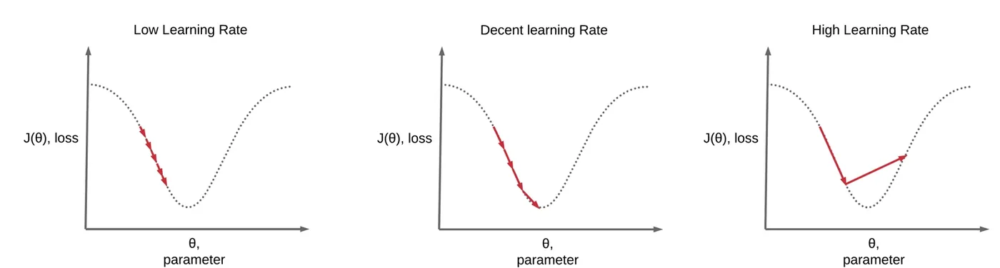
Too small and training crawls. Too big and every step overshoots the bottom and the loss bounces or explodes. A good value descends quickly and settles.
Here it is for real, on the simplest bowl-shaped problem, , whose minimum is at :
import numpy as np
import matplotlib.pyplot as plt

# minimise f(w) = (w - 3)^2, whose slope is 2(w - 3). The true minimum is w = 3.
def descend(lr, steps=25, w=-4.0):
    path = [w]
    for _ in range(steps):
        w = w - lr * 2 * (w - 3)
        path.append(w)
    return np.array(path)

fig, ax = plt.subplots(figsize=(6.6, 3.8))
for lr, color, label in [(0.02, "#F59E0B", "lr = 0.02  too small"),
                         (0.4,  "#16A34A", "lr = 0.4   good"),
                         (1.05, "#DC2626", "lr = 1.05  too big")]:
    p = descend(lr)
    ax.plot((p - 3) ** 2, color=color, lw=2, label=label)
    print(f"{label:24s} loss after 25 steps: {(p[-1] - 3) ** 2:12.4f}")
ax.set_yscale("log"); ax.set_xlabel("step"); ax.set_ylabel("loss (log scale)")
ax.legend(frameon=False); ax.spines[["top", "right"]].set_visible(False)
fig.tight_layout()lr = 0.02 too small loss after 25 steps: 6.3644
lr = 0.4 good loss after 25 steps: 0.0000
lr = 1.05 too big loss after 25 steps: 5752.1518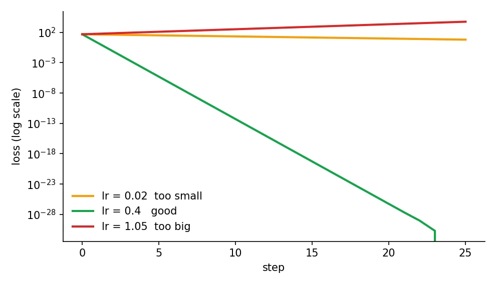
After 25 steps, the cautious rate (0.02) is still at loss 6.4, the good rate (0.4) is down to 0.0000, and the big rate (1.05) has diverged to 5,752. Each step overshoots the minimum by more than it started with, so the error grows instead of shrinking. If your training loss ever goes up and up or turns into nan, suspect the learning rate first.
Batch size
Real datasets are too big to push through the model all at once, so training uses mini-batches. The batch size is how many rows are processed before one parameter update.
- Small batches: many updates per pass and noisy gradients. Cheap on memory.
- Large batches: few updates per pass and smooth gradients. Needs more memory.
- Batch size 1 is true "stochastic" gradient descent, and using the whole dataset is "batch" gradient descent. Session 7 compares them.
The number of updates per pass follows from simple arithmetic:
is the number of training rows and the batch size. The brackets mean "round up", because the last batch may be smaller.
import numpy as np
from sklearn.datasets import load_diabetes
from sklearn.preprocessing import StandardScaler

X, y = load_diabetes(return_X_y=True)
X = StandardScaler().fit_transform(X)
y = (y - y.mean()) / y.std()
n = len(X)

def train(batch_size, epochs=20, lr=0.01, seed=0):
    rng = np.random.default_rng(seed)
    w = np.zeros(X.shape[1]); b = 0.0; updates = 0
    for _ in range(epochs):
        order = rng.permutation(n)
        for i in range(0, n, batch_size):
            idx = order[i:i + batch_size]
            err = y[idx] - (X[idx] @ w + b)
            w += lr * 2 * (X[idx].T @ err) / len(idx)     # gradient step on this mini-batch
            b += lr * 2 * err.mean()
            updates += 1
    return np.mean((y - (X @ w + b)) ** 2), updates

print("batch size   updates in 20 epochs   final loss")
for bs in [1, 32, 353]:
    loss, upd = train(bs)
print(f"{bs:8d} {upd:12d} {loss:.4f}")batch size updates in 20 epochs final loss
1 8840 0.5148
32 280 0.4859
353 40 0.5249With 353 training rows, batch size 1 makes 8,840 updates in 20 passes, batch size 32 makes 280, and the full batch only 40. In this small test the middle option reached the lowest loss (0.486). It is a very common pattern: batch sizes of 16, 32 or 64 are popular defaults because they balance noise, speed and memory.
Epochs
One epoch is one complete pass through the training data. The number of epochs is how many times the model gets to see every row. This hyperparameter links straight to Session 3's two failures:
- Too few epochs: the model has not learned the pattern yet. It does badly on training and validation data (underfitting, high bias). Train longer.
- The right number: training and validation error are both low. This is the sweet spot.
- Too many epochs: the model starts memorising the training rows. Training loss keeps falling while validation loss turns round and climbs (overfitting, high variance).
Let's watch it happen. We train a deliberately oversized small neural network (two layers of 128 neurons, on only about 300 rows) for 300 epochs and record both losses after every epoch.
import numpy as np
import matplotlib.pyplot as plt
from sklearn.datasets import load_diabetes
from sklearn.model_selection import train_test_split
from sklearn.neural_network import MLPRegressor
from sklearn.preprocessing import StandardScaler

X, y = load_diabetes(return_X_y=True)
X = StandardScaler().fit_transform(X)
y = (y - y.mean()) / y.std()
X_tr, X_va, y_tr, y_va = train_test_split(X, y, test_size=0.3, random_state=1)

# a deliberately over-sized network (two layers of 128) on only ~300 rows
net = MLPRegressor(hidden_layer_sizes=(128, 128), learning_rate_init=0.003, alpha=0.0, random_state=0)
train_loss, val_loss = [], []
for epoch in range(300):
    net.partial_fit(X_tr, y_tr)                              # one pass through the training data
    train_loss.append(np.mean((y_tr - net.predict(X_tr)) ** 2))
    val_loss.append(np.mean((y_va - net.predict(X_va)) ** 2))

best = int(np.argmin(val_loss))
print(f"best epoch: {best + 1}   validation loss there: {val_loss[best]:.3f}")
print(f"at epoch 300: train loss {train_loss[-1]:.3f}, validation loss {val_loss[-1]:.3f}")

fig, ax = plt.subplots(figsize=(6.6, 3.8))
ax.plot(train_loss, color="#2563EB", lw=2, label="training loss")
ax.plot(val_loss, color="#F59E0B", lw=2, label="validation loss")
ax.axvline(best, color="#16A34A", ls="--", lw=1.5, label=f"best epoch ({best + 1})")
ax.set_xlabel("epoch"); ax.set_ylabel("loss (MSE)")
ax.legend(frameon=False); ax.spines[["top", "right"]].set_visible(False)
fig.tight_layout()best epoch: 7 validation loss there: 0.479
at epoch 300: train loss 0.000, validation loss 0.769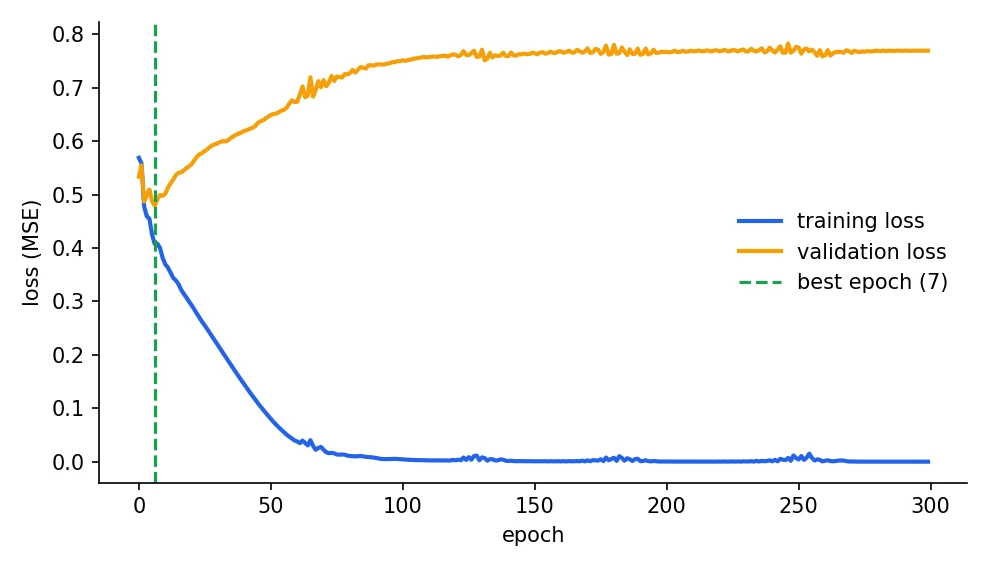
The best validation loss, 0.479, comes at epoch 7. By epoch 300 the training loss has fallen to 0.000, a perfect memorisation of the training rows, while the validation loss has climbed to 0.769, much worse than at epoch 7. Same model, same data. All that changed was how long we trained.
The remedy is early stopping: watch the validation loss, and stop when it has not improved for a set number of epochs (called patience), then keep the best weights. It is free, it works, and it is one of the most useful habits in deep learning.
from tensorflow.keras.callbacks import EarlyStopping

stop = EarlyStopping(monitor="val_loss", patience=5, restore_best_weights=True)
model.fit(X_train, y_train, validation_split=0.2,
          epochs=200, batch_size=32, callbacks=[stop])
The Deep Learning textbook by Goodfellow, Bengio and Courville calls the learning rate "perhaps the most important hyperparameter", and says that if you can tune only one, tune that one.Deep Learning, Goodfellow, Bengio and Courville, 2016
During training, your training loss keeps falling but your validation loss started rising 20 epochs ago. What should you do?
Other hyperparameters you will meet
A quick catalogue. Do not memorise it. Skim so the names ring a bell when each shows up again in its own session.
For neural networks (Sessions 9, 10, 16 to 20):
- Hidden layers and neurons per layer: the depth and width of the network.
- Activation function: ReLU, sigmoid, tanh, softmax (Session 6).
- Optimizer: SGD, Adam, RMSprop, Adagrad (Session 7).
- Momentum: smooths updates so training does not zig-zag.
- Learning-rate decay: shrink the learning rate over time (Session 8).
- Dropout rate: the fraction of neurons switched off at random during training.
- Weight decay / L1 / L2: the penalties from Session 3.
For classical models:
| Model | Key hyperparameters | What they do |
|---|---|---|
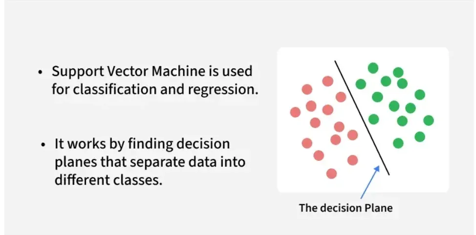
| Logistic regression / SVM | C, penalty |
C is the inverse of regularization strength: smaller means stronger |
| SVM | kernel, gamma |
The shape of the boundary, and how far one point's influence reaches |
| K-nearest neighbours | n_neighbors, metric, weights |
How many neighbours vote, and how distance is measured |
| Decision tree / forest / boosting | max_depth, n_estimators, min_samples_leaf, max_features |
How large and how many trees |
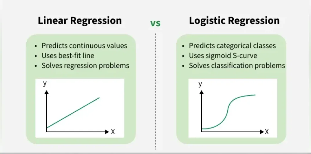
Logistic regression, mentioned there, is the classification cousin of linear regression. It takes the same straight-line score and squeezes it through an S-shaped curve so the output lands between 0 and 1, readable as a probability:
For very negative the output is close to 0, for very positive it is close to 1, and . Logistic regression computes and returns as the probability of the positive class.
from sklearn.linear_model import LogisticRegression
from sklearn.svm import SVC
from sklearn.neighbors import KNeighborsClassifier
from sklearn.ensemble import RandomForestClassifier

LogisticRegression(C=1.0, penalty="l2", max_iter=1000)       # C = inverse regularization strength
SVC(kernel="rbf", C=1.0, gamma="scale")                      # kernel, C, gamma
KNeighborsClassifier(n_neighbors=5, metric="minkowski", weights="distance")
RandomForestClassifier(n_estimators=200, max_depth=8, min_samples_leaf=2, max_features="sqrt")
Everything inside those brackets is a hyperparameter: set before fit, never learned.
How to tune without cheating
There is a trap here, and it is the same one from Session 1. If you try 50 settings, score each on the test set and keep the best, you have used the test set to choose, so its score is no longer an honest surprise. You have leaked test information into your decisions.
The fix is cross-validation (CV) on the training data only. Split the training rows into folds (often 5). Train on 4 folds, validate on the fifth, rotate so every fold gets a turn as the validation set, and average the scores.
is the metric (for example R²) measured on fold when the model was trained on the other folds. The spread across folds (the standard deviation) also matters: it tells you how stable the estimate is.
from sklearn.datasets import load_diabetes
from sklearn.linear_model import Ridge
from sklearn.model_selection import KFold, cross_val_score, train_test_split
from sklearn.pipeline import make_pipeline
from sklearn.preprocessing import StandardScaler

X, y = load_diabetes(return_X_y=True)
X_tr, X_te, y_tr, y_te = train_test_split(X, y, test_size=0.2, random_state=42)

model = make_pipeline(StandardScaler(), Ridge(alpha=10))
cv = KFold(n_splits=5, shuffle=True, random_state=0)
scores = cross_val_score(model, X_tr, y_tr, cv=cv, scoring="r2")

print("R² on each of the 5 folds:", scores.round(3))
print(f"mean {scores.mean():.3f} +/- {scores.std():.3f}")R² on each of the 5 folds: [0.504 0.504 0.573 0.431 0.469]
mean 0.496 +/- 0.047The five folds scored between 0.431 and 0.573, a spread of 0.047. One single split could easily have landed on 0.43 or 0.57 by luck. That is why we trust a CV average more than one split, and why Session 4's advice about not crowning a winner on a 0.01 difference matters.
Grid search
Grid search tries every combination from a grid you define, scoring each with cross-validation. It is exhaustive and simple. Here we tune two things together on a Ridge model: the polynomial degree of the features and the penalty alpha.
import pandas as pd
from scipy.stats import loguniform
from sklearn.datasets import load_diabetes
from sklearn.linear_model import Ridge
from sklearn.model_selection import GridSearchCV, RandomizedSearchCV, train_test_split
from sklearn.pipeline import Pipeline
from sklearn.preprocessing import PolynomialFeatures, StandardScaler

X, y = load_diabetes(return_X_y=True)
X_tr, X_te, y_tr, y_te = train_test_split(X, y, test_size=0.2, random_state=42)

pipe = Pipeline([("poly", PolynomialFeatures(include_bias=False)),
                 ("scale", StandardScaler()),
                 ("ridge", Ridge())])

# Grid search: every combination, 3 x 5 = 15, each scored with 5-fold CV = 75 fits
grid = GridSearchCV(pipe, {"poly__degree": [1, 2, 3], "ridge__alpha": [0.1, 1, 10, 100, 1000]},
                    cv=5, scoring="r2").fit(X_tr, y_tr)
print("GRID   best:", grid.best_params_, "| CV R²:", round(grid.best_score_, 3),
      "| test R²:", round(grid.score(X_te, y_te), 3))

top = pd.DataFrame(grid.cv_results_)[["param_poly__degree", "param_ridge__alpha", "mean_test_score"]]
print(top.sort_values("mean_test_score", ascending=False).head(4).round(3).to_string(index=False))

# Random search: 10 random draws instead of all combinations
rand = RandomizedSearchCV(pipe, {"poly__degree": [1, 2, 3], "ridge__alpha": loguniform(1e-1, 1e4)},
                          n_iter=10, cv=5, scoring="r2", random_state=0).fit(X_tr, y_tr)
print("\nRANDOM best:", {k: (round(v, 1) if isinstance(v, float) else v) for k, v in rand.best_params_.items()},
"| CV R²:", round(rand.best_score_, 3), "| test R²:", round(rand.score(X_te, y_te), 3))GRID best: {'poly__degree': 1, 'ridge__alpha': 10} | CV R²: 0.454 | test R²: 0.457
param_poly__degree param_ridge__alpha mean_test_score
1 10 0.454
1 1 0.451
1 100 0.451
1 0.1 0.450
RANDOM best: {'poly__degree': 1, 'ridge__alpha': 8.3} | CV R²: 0.454 | test R²: 0.457Three results are worth reading slowly.
- The winner uses degree 1, a plain straight line, with
alpha = 10. The fancier polynomial features did not help, they overfit. Tuning is not about picking the most complex model, it is about finding the right amount. - The CV score of the best model (0.454) is almost the same as its test score (0.457). That agreement is the sign of an honest process: the test set was used exactly once, at the end.
- That grid had 3 x 5 = 15 combinations, each trained 5 times: 75 fits. A grid grows fast. Add a third hyperparameter with 5 values and it is 375 fits.
Random search
Random search samples a fixed number of random combinations instead. It looks less thorough but it is often better, because usually only one or two hyperparameters really matter, and random sampling tests many different values of each one rather than repeating the same few. Above, 10 random draws (about two-thirds of the grid's work) found alpha = 8.3 and the same CV score of 0.454.
A third family, Bayesian optimisation (tools such as Optuna), uses the results of earlier trials to decide where to look next. It pays off when each trial is expensive, like training a big neural network.
| Method | Idea | Best when |
|---|---|---|
| Grid search | Try every combination | Few hyperparameters, few values |
| Random search | Try random combinations | Many hyperparameters, limited time |
| Bayesian optimisation | Learn from earlier trials | Each trial is slow or costly |
from sklearn.model_selection import GridSearchCV, RandomizedSearchCV
from sklearn.ensemble import RandomForestRegressor

grid = GridSearchCV(RandomForestRegressor(random_state=0),
                    param_grid={"n_estimators": [100, 200], "max_depth": [None, 5, 10]},
                    cv=5, scoring="r2")
grid.fit(X_train, y_train)
print(grid.best_params_, grid.best_score_)
# RandomizedSearchCV(estimator, param_distributions, n_iter=20, cv=5) samples insteadscikit-learn, the library behind most code in Part I, began in 2007 as a Google Summer of Code project by David Cournapeau. Today it is one of the most widely used machine learning libraries in Python.scikit-learn project history
You tried 40 hyperparameter settings and kept the one with the best test-set score. What is the problem?
Try it yourself
- In
learning_rate.py, trylr = 0.9andlr = 1.0. What is special about exactly 1.0 on this problem? (Hint: look at the update formula.) - In
epochs.py, addalpha=0.5to theMLPRegressor(that is its L2 penalty). Does the best epoch move? Does validation loss still climb? - Extend the grid in
grid_random.pywithdegree 4. What happens to the CV score? Why? - Write a loop that fits a random forest with
max_depthfrom 1 to 12 and plots training and validation R² against depth. Where does overfitting begin?
Part I complete: what you can do now
Stop for a second. You can set up an environment, clean and split data without leaking, train a line, fix its overfitting with Ridge and Lasso, score it with the right metric and tune its settings honestly. That is the same workflow a professional uses, only on small data.
Part II opens the engine room. Session 6 looks at what "wrong" means to a model (loss functions) and how curves enter the picture (activation functions). That is where neural networks begin to make sense.
Frequently asked questions
What is the difference between a parameter and a hyperparameter?
Parameters are learned from the data during training, like the weights of a neural network or the slope of a line. Hyperparameters are chosen by you before training, like the learning rate, batch size, number of epochs or tree depth. The model never changes its own hyperparameters.
How many epochs should I train for?
There is no fixed number. Train with a validation set, watch the validation loss, and use early stopping to halt when it stops improving. In our example the best epoch was 7 out of 300, but it depends on the model and the data.
What is a good batch size?
Common defaults are 16, 32 or 64. Smaller batches give noisier updates and use less memory, larger ones are smoother and faster per epoch on a GPU but need more memory. It also interacts with the learning rate, so if you change one, check the other.
Is grid search or random search better?
Grid search is fine when you have only a couple of hyperparameters with a few values each. Random search usually finds equally good settings with less work when there are many hyperparameters, because it explores more distinct values of each one.
Why can't I tune hyperparameters on the test set?
Because choosing the best of many settings by its test score makes the test score optimistic, since the test data has influenced your decision. Use cross-validation on the training data to tune, and keep the test set for one final check.