
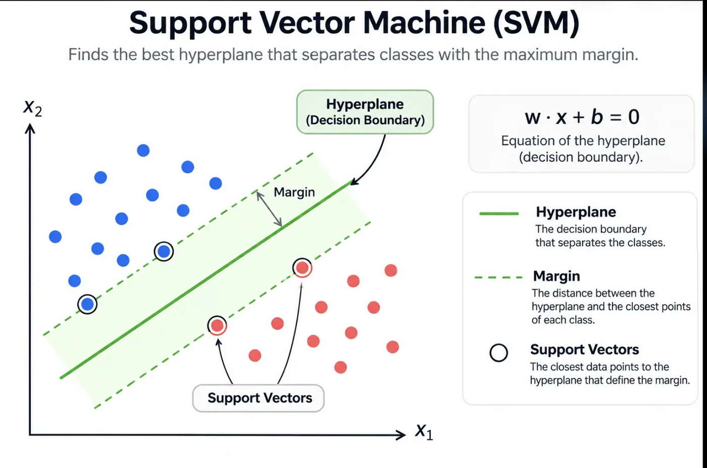
Suppose you have two groups of points and many different straight lines that separate them perfectly. Which line should you pick? A support vector machine (SVM) has a clear answer: pick the one that sits as far as possible from both groups, the line with the widest empty street between them. That street is called the margin, and the idea that a wide margin generalises better is the whole philosophy of the model.
Trees (Sessions 11 to 13) split data with questions. SVMs think in geometry instead, and with one clever trick, the kernel, they can draw curved boundaries too. This session explains the margin, the support vectors, the kernel trick and the two settings you will tune most, C and gamma. It uses the hinge loss from Session 6 and the hyperparameter ideas of Session 5.
The vocabulary
- Hyperplane: the decision boundary. In two dimensions it is a line, in three a flat plane, in more dimensions a hyperplane.
- Margin: the gap between the boundary and the nearest points of each class. The SVM maximises it.
- Support vectors: the points closest to the boundary. They are the only points that matter: move any other point and the boundary does not change.
- Kernel trick: a way to separate data that no straight line can split.
- Soft margin and C: permission to misclassify a few points when the classes overlap.
The maths of the maximum margin
A hyperplane is the set of points where . A new point is classified by which side it lands on. The two edges of the margin sit where the expression equals and , and the distance between them is . So maximising the margin means minimising the length of .
Here is the class label, or . The constraint says every point must be on the correct side and at least a margin away. The margin width is , so a smaller means a wider street. This is only possible if the classes can be separated perfectly.
Real data overlaps, so we allow some points to cross the margin by paying a price. Each violation gets a slack , and the constant sets how expensive violations are:
Large : mistakes are costly, so the model fights to classify every training point correctly, with a narrow margin (risk of overfitting). Small : mistakes are cheap, so it accepts a wider margin with more errors (risk of underfitting). Note that works like from Session 3: a smaller means stronger regularisation.
The same thing can be written as the hinge loss from Session 6, so an SVM is a linear model trained with a particular loss and an L2 penalty:
If a point is correct and beyond the margin () the loss is exactly 0, so it has no influence at all. Only points on or inside the margin contribute, and those are the support vectors.
Here it is in code, on two clusters of points with a very large (nearly a hard margin):
import numpy as np
import matplotlib.pyplot as plt
from sklearn.datasets import make_blobs
from sklearn.svm import SVC

X, y = make_blobs(n_samples=60, centers=[(-2, -1.5), (2, 1.5)], cluster_std=1.1, random_state=4)
svm = SVC(kernel="linear", C=1000).fit(X, y)            # a very large C = (nearly) a hard margin
w, b = svm.coef_[0], svm.intercept_[0]
print("weights w:", w.round(3), "  bias b:", round(b, 3))
print("margin width = 2 / ||w|| =", round(2 / np.linalg.norm(w), 3))
print("support vectors:", len(svm.support_vectors_), "of", len(X), "points")

xs = np.linspace(-5, 5, 50)
line = lambda c: -(w[0] * xs + b - c) / w[1]
fig, ax = plt.subplots(figsize=(6.2, 4))
ax.scatter(X[:, 0], X[:, 1], c=y, cmap="coolwarm", s=28)
ax.scatter(*svm.support_vectors_.T, s=160, facecolors="none", edgecolors="k", linewidths=1.6, label="support vectors")
ax.plot(xs, line(0), "k-", lw=2, label="decision boundary"); ax.plot(xs, line(1), "k--", lw=1); ax.plot(xs, line(-1), "k--", lw=1)
ax.set_ylim(-5, 5); ax.set_xlim(-5, 5); ax.legend(frameon=False, loc="lower right"); ax.spines[["top", "right"]].set_visible(False)
fig.tight_layout()weights w: [1.206 2.342] bias b: -0.202
margin width = 2 / ||w|| = 0.759
support vectors: 3 of 60 points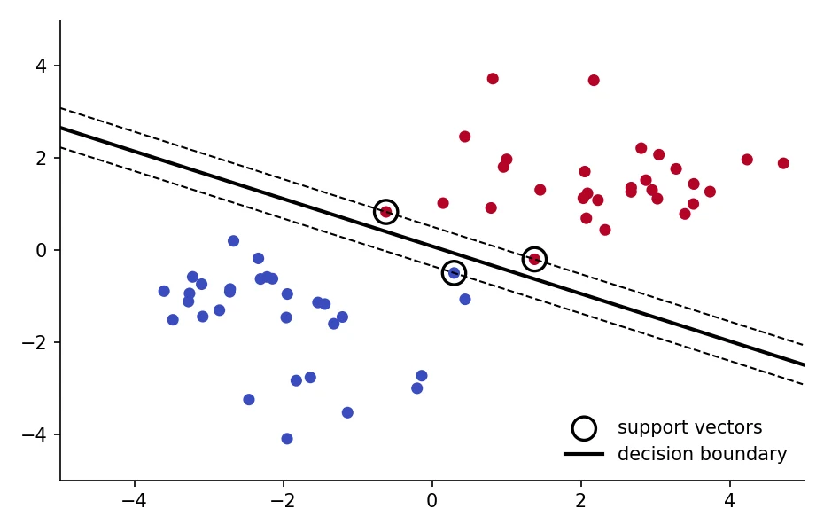
The model found weights and a margin width of . And look at the last line: only 3 of the 60 points are support vectors. The other 57 could be deleted and the boundary would not move at all. In the figure, the three circled points touch the dashed margin lines.
The soft-margin SVM was published by Corinna Cortes and Vladimir Vapnik in 1995. The kernel trick for SVMs came three years earlier, from Boser, Guyon and Vapnik in 1992. Vapnik and Chervonenkis laid the theory in the 1960s.Cortes and Vapnik, Machine Learning, 1995
In a trained SVM, which training points determine the position of the decision boundary?
The kernel trick: bending the boundary
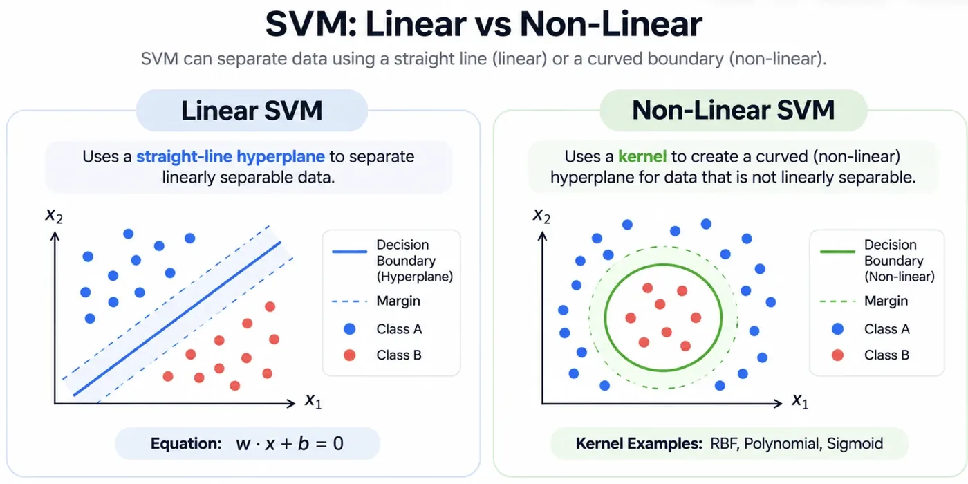
A straight boundary fails when the classes are tangled, like a ring of points around a core. The insight behind the kernel trick is that data that cannot be separated in one space can often be separated if you lift it into a higher dimension.
Take points on a line: class 1 on the outer edges, class 0 in the middle. No single cut on the line separates them. Now add a new feature, the square of the position. In two dimensions (position and its square) the middle points sit low and the outer points sit high, and a flat line separates them.
import numpy as np
import matplotlib.pyplot as plt
from sklearn.svm import SVC

x = np.array([-4, -3, -2, -1, 0, 1, 2, 3, 4], dtype=float)
y = (np.abs(x) > 2).astype(int)                     # class 1 is on the outside, class 0 in the middle

print("on the original line, a single cut cannot separate them:")
print("  best straight-line (linear) SVM accuracy:", SVC(kernel="linear").fit(x.reshape(-1, 1), y).score(x.reshape(-1, 1), y).round(3))
X2 = np.column_stack([x, x ** 2])                   # add one new feature: x squared
print("after adding the feature x², a straight line separates them:")
print("  linear SVM accuracy in 2D:", SVC(kernel="linear", C=100).fit(X2, y).score(X2, y))

fig, ax = plt.subplots(1, 2, figsize=(9, 3.2))
ax[0].scatter(x, np.zeros_like(x), c=y, cmap="coolwarm", s=70); ax[0].set_yticks([]); ax[0].set_title("1D: no single cut works")
ax[1].scatter(X2[:, 0], X2[:, 1], c=y, cmap="coolwarm", s=70); ax[1].axhline(5, color="k", lw=1.5)
ax[1].set_title("add x²: a straight line splits them"); ax[1].set_xlabel("x"); ax[1].set_ylabel("x²")
for a in ax: a.spines[["top", "right"]].set_visible(False)
fig.tight_layout()on the original line, a single cut cannot separate them:
best straight-line (linear) SVM accuracy: 0.556
after adding the feature x², a straight line separates them:
linear SVM accuracy in 2D: 1.0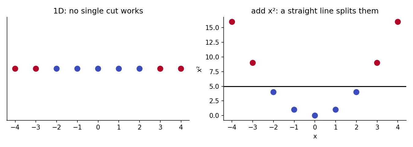
A linear SVM on the original line scores 0.556, barely better than chance. After adding , a straight line gets it 100 percent right. The kernel trick takes this further: it computes what the SVM needs in the high-dimensional space without ever building those extra coordinates, using only a function of pairs of points. The most popular choice is the RBF kernel.
It measures similarity: 1 when two points coincide, falling towards 0 as they move apart. ("gamma") controls how fast: a large means each point's influence is very local (a wiggly boundary), a small means influence reaches far (a smooth boundary). It implicitly works in an infinite-dimensional space.
(The Radial Basis Function is the name. It is not a "bias" function, a slip you may see in some notes.)
The common kernels are linear (a plain straight boundary), polynomial (curves like and ), RBF (the default choice for curved data) and sigmoid.
import numpy as np
import matplotlib.pyplot as plt
from sklearn.datasets import make_moons
from sklearn.model_selection import train_test_split
from sklearn.svm import SVC

X, y = make_moons(n_samples=300, noise=0.25, random_state=1)
X_tr, X_te, y_tr, y_te = train_test_split(X, y, test_size=0.3, random_state=1)

gx, gy = np.meshgrid(np.linspace(-2, 3, 250), np.linspace(-1.5, 2, 250))
fig, ax = plt.subplots(1, 3, figsize=(11, 3.3), sharey=True)
for a, (name, svm) in zip(ax, [("linear", SVC(kernel="linear")), ("polynomial (degree 3)", SVC(kernel="poly", degree=3, coef0=1)), ("RBF", SVC(kernel="rbf", gamma=1))]):
    svm.fit(X_tr, y_tr)
    acc = svm.score(X_te, y_te)
    print(f"{name:22s} test accuracy {acc:.3f}   support vectors {svm.n_support_.sum()}")
    a.contourf(gx, gy, svm.predict(np.c_[gx.ravel(), gy.ravel()]).reshape(gx.shape), cmap="coolwarm", alpha=.25)
    a.scatter(X_tr[:, 0], X_tr[:, 1], c=y_tr, cmap="coolwarm", s=12, edgecolors="none")
    a.set_title(f"{name}  ({acc:.2f})"); a.spines[["top", "right"]].set_visible(False)
fig.tight_layout()linear test accuracy 0.822 support vectors 76
polynomial (degree 3) test accuracy 0.933 support vectors 53
RBF test accuracy 0.944 support vectors 61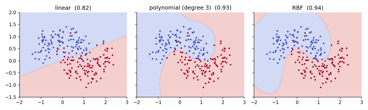
On two interleaved moons with noise, the linear kernel scores only 0.822 on unseen points. The polynomial kernel gets 0.933 and the RBF kernel 0.944. Same algorithm, same data, different geometry. The figure shows the linear boundary as a straight cut and the other two bending around the crescents.
Tuning C and gamma
With the RBF kernel, two hyperparameters decide everything: (how much to punish training mistakes) and (how local each point's influence is). Here is a 3 by 3 grid of settings on noisy moons.
import numpy as np
import matplotlib.pyplot as plt
from sklearn.datasets import make_moons
from sklearn.model_selection import train_test_split
from sklearn.svm import SVC

X, y = make_moons(n_samples=300, noise=0.3, random_state=2)
X_tr, X_te, y_tr, y_te = train_test_split(X, y, test_size=0.3, random_state=2)
gx, gy = np.meshgrid(np.linspace(-2, 3, 200), np.linspace(-1.5, 2, 200))

fig, ax = plt.subplots(3, 3, figsize=(9.5, 8), sharex=True, sharey=True)
print("   C    gamma   train   test")
for i, C in enumerate([0.1, 1, 100]):
    for j, gamma in enumerate([0.1, 1, 30]):
        svm = SVC(kernel="rbf", C=C, gamma=gamma).fit(X_tr, y_tr)
        tr, te = svm.score(X_tr, y_tr), svm.score(X_te, y_te)
        print(f"{C:5g}  {gamma:5g}   {tr:.3f}   {te:.3f}")
        a = ax[i, j]
        a.contourf(gx, gy, svm.predict(np.c_[gx.ravel(), gy.ravel()]).reshape(gx.shape), cmap="coolwarm", alpha=.25)
        a.scatter(X_tr[:, 0], X_tr[:, 1], c=y_tr, cmap="coolwarm", s=8, edgecolors="none")
        a.set_title(f"C={C}, gamma={gamma}", fontsize=9); a.set_xticks([]); a.set_yticks([])
fig.tight_layout() C gamma train test
0.1 0.1 0.843 0.722
0.1 1 0.886 0.811
0.1 30 0.586 0.500
1 0.1 0.862 0.756
1 1 0.905 0.867
1 30 0.938 0.878
100 0.1 0.905 0.833
100 1 0.924 0.867
100 30 1.000 0.822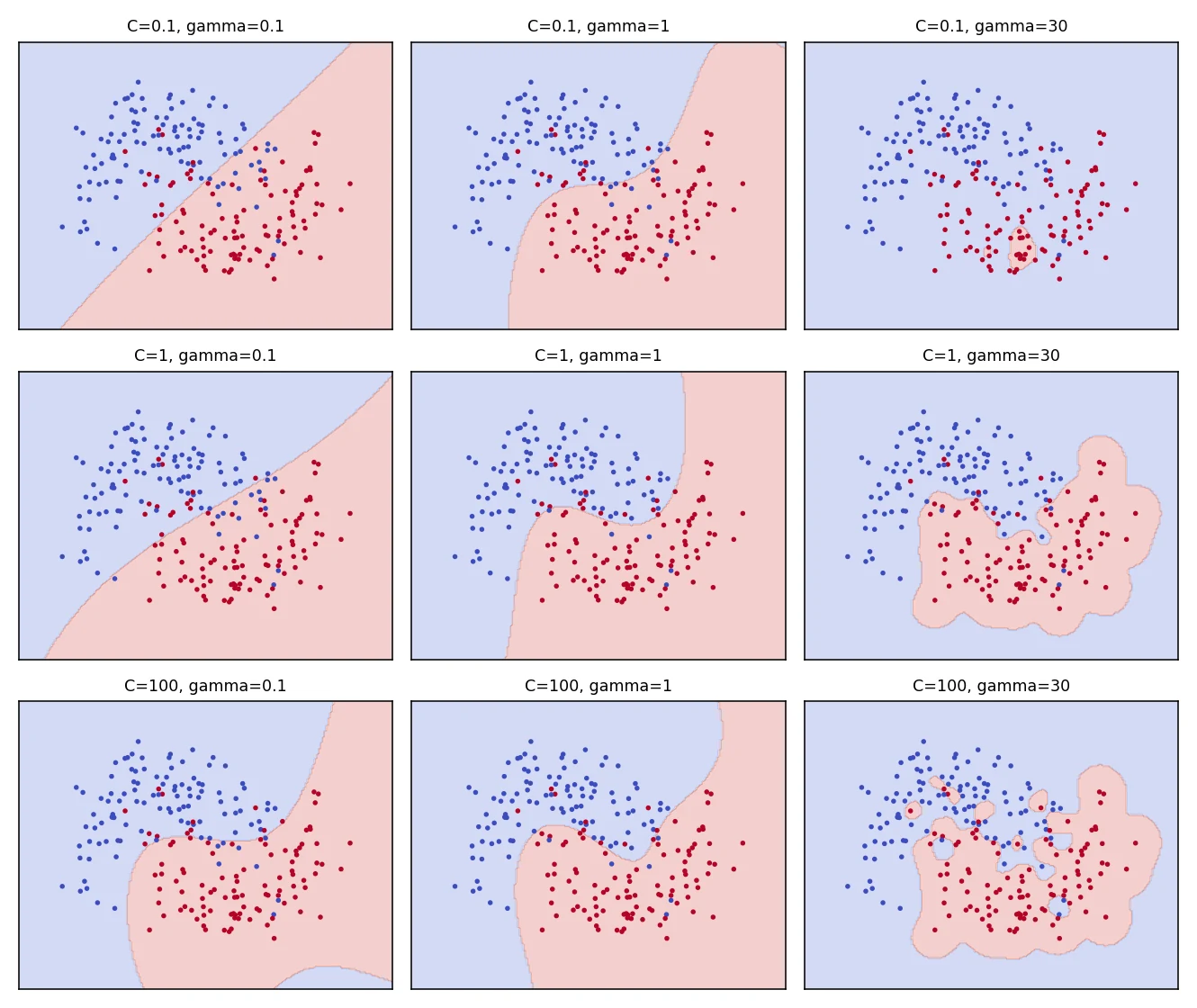
The table tells the story. Top row, C = 0.1: the model is tightly regularised. With gamma = 30 it fails outright, a train accuracy of 0.586 and a test accuracy of 0.500, no better than chance. Middle row, C = 1: with gamma = 1 or 30 it reaches a test accuracy of 0.867 to 0.878, the best region. Bottom row, C = 100: with gamma = 30 the training accuracy hits a perfect 1.000 but the test accuracy falls to 0.822, the unmistakable look of overfitting: a boundary that wraps individual points. In practice you search for the best pair with cross-validation (Session 5), usually on a logarithmic scale such as 0.01, 0.1, 1, 10, 100.
The one thing you must not forget: scale your features
An SVM relies on distances, so a feature measured in thousands can swamp one measured in fractions. Always scale, and keep the scaler in a pipeline so it only ever sees training data.
from sklearn.datasets import load_breast_cancer
from sklearn.model_selection import cross_val_score
from sklearn.pipeline import make_pipeline
from sklearn.preprocessing import StandardScaler
from sklearn.svm import SVC

X, y = load_breast_cancer(return_X_y=True)
print("feature ranges differ a lot: smallest column max =", X.max(axis=0).min().round(3), " largest column max =", X.max(axis=0).max().round(1))
raw = cross_val_score(SVC(kernel="rbf"), X, y, cv=5).mean()
scaled = cross_val_score(make_pipeline(StandardScaler(), SVC(kernel="rbf")), X, y, cv=5).mean()
print(f"SVM without scaling: {raw:.3f}")
print(f"SVM with scaling   : {scaled:.3f}")

svm = make_pipeline(StandardScaler(), SVC(kernel="rbf", C=1.0, gamma="scale")).fit(X, y)
print("support vectors (points that define the boundary):", svm[-1].support_vectors_.shape[0], "of", len(X))feature ranges differ a lot: smallest column max = 0.03 largest column max = 4254.0
SVM without scaling: 0.912
SVM with scaling : 0.974
support vectors (points that define the boundary): 119 of 569In the breast-cancer data, the largest value in one column is 4,254 while in another it is 0.03. Without scaling the SVM scores 0.912, and with a scaler it jumps to 0.974, a gain of six points from one line of preprocessing. The last line shows the final model uses 119 of the 569 rows as support vectors.
from sklearn.pipeline import make_pipeline
from sklearn.preprocessing import StandardScaler
from sklearn.svm import SVC

svm = make_pipeline(StandardScaler(), SVC(kernel="rbf", C=1.0, gamma="scale"))
svm.fit(X_train, y_train)
print(svm.score(X_test, y_test))
print(svm[-1].support_vectors_.shape)     # the points that define the boundary
SVC is for classification and SVR does regression. For probabilities add probability=True, which is slower.
Strengths and weaknesses
| Strengths | Weaknesses |
|---|---|
| Works well in high dimensions, even with more features than rows | Slow to train on large datasets |
| Flexible through kernels (linear, polynomial, RBF) | Needs careful tuning of the kernel, and |
| Memory-efficient: stores only support vectors | Sensitive to feature scaling |
| Soft margin tolerates some outliers and overlap | Hard to interpret, and no direct probabilities |
| Strong on small to medium datasets, text and gene data | Struggles when classes overlap heavily or the data is very noisy |
You train an RBF SVM and get 100 percent training accuracy but poor test accuracy. Which change is most likely to help?
Try it yourself
- In
margin.py, add one extra point far inside the wrong class. WithC=1000and thenC=0.1, how does the boundary move? - In
kernels_compare.py, changedegree=3todegree=8. What happens to the polynomial accuracy? - In
c_gamma.py, add a tenth setting of your own and try to beat 0.878 on the test set. - Fit an
SVRon the diabetes data (with scaling) and compare its test R² with the earlier models.
What comes next
We have now seen four ways to build a classifier on tables: linear models, single trees, forests and boosting, and the SVM. A natural question is whether we should pick the best one or use them all together. Session 15 answers it: ensembles of different models, including stacking, and an honest look at when the extra effort is worth it.
Frequently asked questions
What is a support vector machine in simple terms?
It is a classifier that finds the boundary with the widest possible margin between two classes. Only the points nearest the boundary, called support vectors, decide where it sits. With kernels it can also draw curved boundaries.
What is the kernel trick?
Data that cannot be separated by a straight line may be separable after mapping it into a higher-dimensional space. The kernel trick computes the similarity between points as if they were in that space without actually creating the extra coordinates, so it is fast even for very high or infinite dimensions.
What do C and gamma do in an SVM?
C controls how strongly training errors are penalised: large C gives a narrow margin and fewer training mistakes, small C a wider margin and more tolerance. Gamma, in the RBF kernel, controls how far each point's influence reaches: large gamma gives a wiggly local boundary, small gamma a smooth one. Tune both with cross-validation.
Do SVMs need feature scaling?
Yes. SVMs depend on distances between points, so features on larger scales dominate. Standardise the features inside a pipeline before training.
When should I choose an SVM over a random forest or XGBoost?
SVMs are a strong choice for small to medium datasets with many features, such as text or gene data, and when you want a clean maximum-margin boundary. On large tabular datasets, tree ensembles are usually faster to train and need less preprocessing.