Almost every beginner I know lost their first week to the same thing. Not maths, not algorithms. A broken install, a notebook that cannot find pandas, a CSV that loads with the wrong columns. Then the model "works" in the notebook and fails the moment it sees new data, and nobody can say why.
This first session is about getting that ground solid. By the end you will have a working Python setup, a real medical dataset loaded and cleaned, a train/test split you can trust, and a clear picture of what "training a model" actually means. Every code block below was run for this article, and the output you see is the real output.
If you want the whole map before you start, the full AI and machine learning roadmap shows where this session sits. It is the first of 30, and nothing earlier is needed.
What you need before you start
Three things, none of them expensive:
- A computer with about 4 GB of free space. Any laptop from the last eight years is fine for this whole Part.
- A Python install, version 3.10 or newer. Check with
python --versionin a terminal. - A habit of running code yourself. Reading is not enough here, you learn by changing a number and seeing what breaks.
No GPU is needed until Part IV (images and sequences). If your laptop is slow, Google Colab gives you a free notebook in the browser with nothing to install, and it is how a lot of students in Pakistan start. The code in this article runs there without changes.
Set up your environment the clean way
The single best habit is to give every project its own virtual environment. It is a private folder of packages, so installing something for one project cannot break another.
python -m venv ml-env
source ml-env/bin/activate          # Windows: ml-env\Scripts\activate
pip install numpy pandas matplotlib scikit-learn joblib jupyterlab
jupyter lab
That last line opens JupyterLab in your browser. A notebook is a document where you write code in small cells and see each result straight away, which is why data people live in them. If you prefer an editor, VS Code runs notebooks too.
Later sessions add torch, transformers and friends. Install those only when a session needs them. A bloated environment is slower and harder to repair.
Once it is running, confirm what you actually have. Library versions matter because APIs change between releases, so when something behaves differently from a tutorial, the version is the first suspect.
import sys
import numpy, pandas, sklearn, matplotlib

print("Python      ", sys.version.split()[0])
print("NumPy       ", numpy.__version__)
print("pandas      ", pandas.__version__)
print("scikit-learn", sklearn.__version__)
print("matplotlib ", matplotlib.__version__)Python 3.11.14
NumPy 1.26.4
pandas 2.3.3
scikit-learn 1.2.2
matplotlib 3.10.1Your numbers may be newer than mine, and that is fine. Everything here works on current releases of these libraries.
Python is named after the British comedy group Monty Python, not the snake. Guido van Rossum released the first version in 1991.
The data you will use
We will use the diabetes dataset that ships inside scikit-learn, so there is nothing to download. It has 442 patients. For each one there are ten baseline measurements (age, sex, body mass index, average blood pressure and six blood-serum readings) and one number we want to predict: a score of how much the disease progressed one year later. It comes from the 2004 paper Least Angle Regression by Efron, Hastie, Johnstone and Tibshirani.
One detail trips people up. The ten feature columns in this copy are already mean-centred and scaled, which is why age looks like 0.038 and not 59. The target was left alone. Keep that in mind when you read the output.
import matplotlib.pyplot as plt
import pandas as pd

pd.set_option("display.width", 120)
from sklearn.datasets import load_diabetes

data = load_diabetes(as_frame=True)
df = data.frame            # 10 feature columns + the target column
print(df.shape)
print(df.head(3).round(3))
print()
print(df["target"].describe().round(1))

fig, ax = plt.subplots(1, 2, figsize=(10, 3.6))
ax[0].hist(df["target"], bins=25, color="#2563EB", edgecolor="white")
ax[0].set_title("Target: disease progression after 1 year")
ax[0].set_xlabel("score"); ax[0].set_ylabel("patients")
ax[1].scatter(df["bmi"], df["target"], s=12, alpha=.6, color="#7C3AED")
ax[1].set_title("bmi (scaled) vs target")
ax[1].set_xlabel("bmi"); ax[1].set_ylabel("target")
for a in ax: a.spines[["top", "right"]].set_visible(False)
fig.tight_layout()(442, 11)
age sex bmi bp s1 s2 s3 s4 s5 s6 target
0 0.038 0.051 0.062 0.022 -0.044 -0.035 -0.043 -0.003 0.020 -0.018 151.0
1 -0.002 -0.045 -0.051 -0.026 -0.008 -0.019 0.074 -0.039 -0.068 -0.092 75.0
2 0.085 0.051 0.044 -0.006 -0.046 -0.034 -0.032 -0.003 0.003 -0.026 141.0
count 442.0
mean 152.1
std 77.1
min 25.0
25% 87.0
50% 140.5
75% 211.5
max 346.0
Name: target, dtype: float64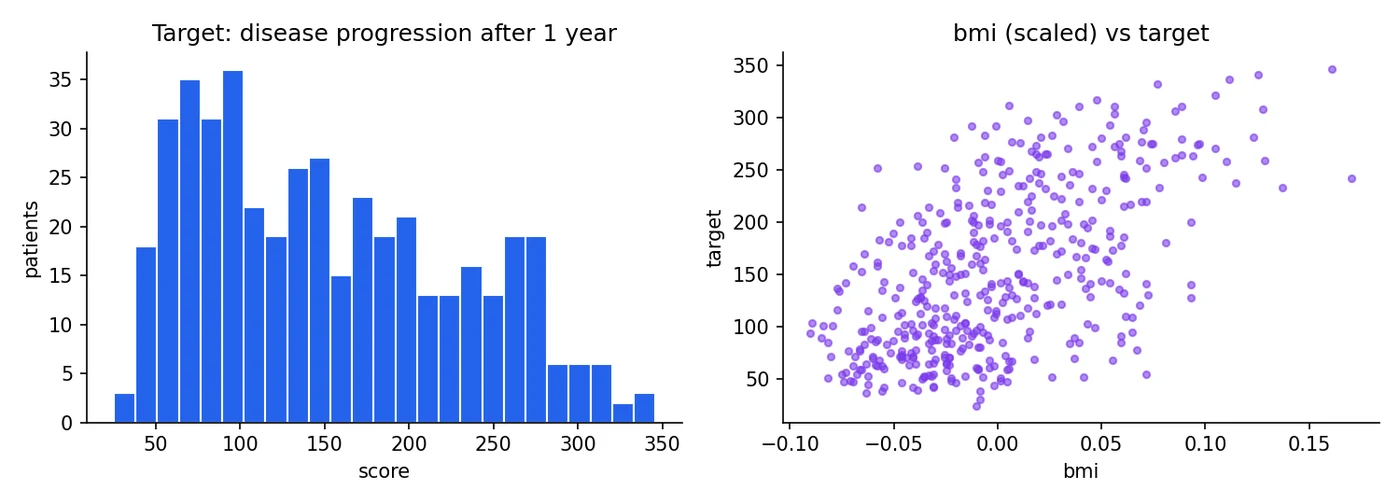
Two things to notice. First, 442 rows and 11 columns: ten features and one target. Second, the picture. The target is spread from about 25 to 346, and patients with a higher BMI tend to sit higher on the progression score. That upward drift is the pattern we will teach a model to find in Session 2.
Features, target and the vocabulary you will hear everywhere
The ten measurements are the features (also called inputs or independent variables). The progression score is the target (also called the label or dependent variable). A model is a function that learns to turn features into a target.
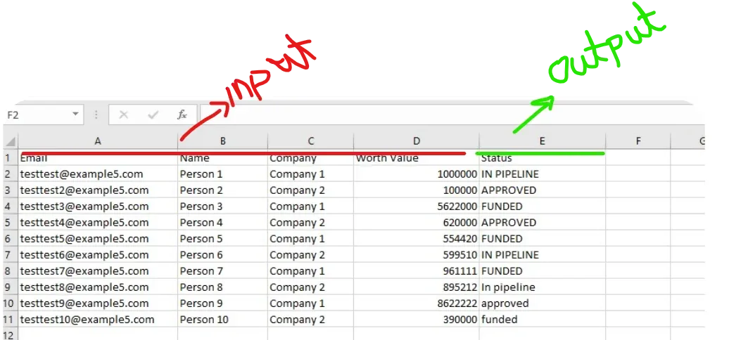
We use X for the feature table and y for the target. Capital X because it is a table, lowercase y because it is a single column. You will see this in nearly every tutorial.
Look before you model: EDA and cleaning
Exploratory data analysis (EDA) is just looking at your data with suspicion before any model touches it. A short checklist that catches most problems:
- How many rows and columns? Is that what you expected?
- What are the types? Numbers stored as text will quietly break things.
- How many values are missing, and in which columns?
- Are there duplicate rows?
- Do any values look impossible? A student who studied 40 hours in one day is a typo or a lie.
- How is each column distributed? Histograms and
describe()tell you fast.
The diabetes data is already clean, so here is a deliberately messy table of the kind you get from a school spreadsheet. It has a missing city, a missing number, a duplicated student and an impossible value.
import numpy as np
import pandas as pd

pd.set_option("display.width", 120)
pd.set_option("display.max_columns", 20)

# A small, deliberately messy table, the kind you really get from a spreadsheet
df = pd.DataFrame({
    "student": ["Ali", "Sara", "Bilal", "Hina", "Sara", "Usman", "Zainab", "Omar"],
    "city":    ["Lahore", "Karachi", "Lahore", "Peshawar", "Karachi", None, "Quetta", "Lahore"],
    "study_hours": [4.0, 6.5, np.nan, 5.0, 6.5, 3.0, 7.0, 40.0],
    "marks":   [62, 81, 55, 74, 81, 49, 88, 70],
})

print("Missing values per column:")
print(df.isna().sum())

df = df.drop_duplicates()                                         # Sara appears twice
df["city"] = df["city"].fillna("Unknown")                         # a category gets a label
df["study_hours"] = df["study_hours"].fillna(df["study_hours"].median())  # a number gets the median

# 40 hours of study in one day is not possible -> outlier. IQR rule:
q1, q3 = df["study_hours"].quantile([0.25, 0.75])
iqr = q3 - q1
mask = df["study_hours"].between(q1 - 1.5 * iqr, q3 + 1.5 * iqr)
print("\nRows flagged as outliers:", df.loc[~mask, "student"].tolist())
df = df[mask]

# Models need numbers, so one-hot encode the text column
X = pd.get_dummies(df[["city", "study_hours"]], columns=["city"], dtype=int)
print("\nModel-ready features:")
print(X)Missing values per column:
student 0
city 1
study_hours 1
marks 0
dtype: int64
Rows flagged as outliers: ['Omar']
Model-ready features:
study_hours city_Karachi city_Lahore city_Peshawar city_Quetta city_Unknown
0 4.00 0 1 0 0 0
1 6.50 1 0 0 0 0
2 5.75 0 1 0 0 0
3 5.00 0 0 1 0 0
5 3.00 0 0 0 0 1
6 7.00 0 0 0 1 0Read the choices in that code, because each one is a decision and not a rule. A missing number got the median, since the median is not dragged around by extreme values the way the mean is. A missing category got its own label, Unknown, because guessing a city would invent facts. The outlier was found with the IQR rule: anything more than 1.5 times the inter-quartile range outside the middle half of the data is flagged. Flagged does not mean deleted automatically. Here 40 study hours is clearly an error, so it goes. A genuine unusual value, like a 99th-percentile house price, should usually stay.
Then one-hot encoding. A model cannot do arithmetic on the word "Lahore", so each city becomes its own 0/1 column. That is what pd.get_dummies did above.
Daily prices are a sequence, and the future must never leak into the past. For that kind of data you split by time (train on earlier dates, test on later ones) and you never shuffle. The random split below is for rows that are independent of each other, like patients.
Training data and testing data
Here is the idea that holds the whole field up. If you grade a student with the exact questions they practised on, the mark tells you about their memory, not their understanding. Models are the same. So we hold some data back, never show it during training, and use it at the end as an honest exam.
- Training set: the rows the model learns from. Typically 70 to 80 percent.
- Test set: rows kept hidden until the very end. Typically 20 to 30 percent.
A third piece, the validation set, appears once you start tuning settings (Session 5). You tune on validation and report on test, so the test set stays a true surprise.
from sklearn.datasets import load_diabetes
from sklearn.linear_model import LinearRegression
from sklearn.model_selection import train_test_split
from sklearn.pipeline import make_pipeline
from sklearn.preprocessing import StandardScaler

X, y = load_diabetes(return_X_y=True)

X_train, X_test, y_train, y_test = train_test_split(
    X, y, test_size=0.2, random_state=42)
print("train:", X_train.shape, " test:", X_test.shape)

# Right way: the scaler only ever sees the training rows, even inside cross-validation
model = make_pipeline(StandardScaler(), LinearRegression())
model.fit(X_train, y_train)
print("R² on data the model never saw:", round(model.score(X_test, y_test), 3))train: (353, 10) test: (89, 10)
R² on data the model never saw: 0.453random_state=42 makes the shuffle repeatable, so you and I get the same split. The number 42 means nothing, it is just a fixed seed.
That R² of 0.453 is a real score on 89 patients the model never saw. We will unpack R² properly in Session 4. For now just read it as "the model explains a bit under half of the variation", which for ten basic measurements is respectable.
The mistake that fools experts: data leakage
Look at how the scaling was done in that code. Standardising a column means subtracting its mean and dividing by its standard deviation:
is the column's mean and its standard deviation. After this, a column has mean 0 and spread 1, so no feature shouts louder than the others just because its units are bigger.
The trap is calculating and on the whole dataset before splitting. The test rows then influenced the numbers used to prepare the training rows. Information leaked from the exam paper into the study notes, and your score comes out better than it deserves. Putting the scaler inside a Pipeline, as above, means it is fitted on training rows only, every time.
You standardise the full dataset with StandardScaler and only then call train_test_split. What went wrong?
How a model actually trains
Ignore the fancy names for a moment. Training is a loop with four steps, and every model in this course, from a straight line to a model with billions of weights, uses a version of it:
- Forward pass. The model makes a guess using its current numbers.
- Loss. A function measures how wrong the guess was.
- Gradients. Work out, for each number inside the model, which direction would make the loss smaller.
- Update. Nudge every number a little in that direction. Repeat.
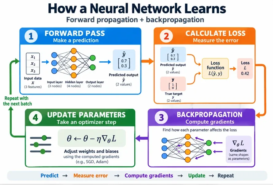
The popular names are "forward propagation" for step 1 and "backpropagation" for steps 3 and 4. We take them apart properly in Session 10. For now it is enough to see the loop run on real data, so here is the smallest possible version: one feature (BMI), two numbers to learn, and about ten lines of NumPy.
The model is a straight line, where is the slope and the intercept:
is the input, ("y-hat") is the guess, and and are the parameters the loop will learn.
The loss is the mean squared error. Take each mistake, square it so that over- and under-shooting both count and big mistakes count extra, then average:
is the number of rows, the true value and the prediction for row . Lower is better, and zero would mean every guess was perfect.
And the update rule, which is gradient descent in one line. Each parameter moves a small step against its slope on the loss. The step size ("eta", the learning rate) is a setting we choose:
For our straight line, . The minus sign inside matters: it is what makes the update push in the direction that reduces the loss.
import numpy as np
import matplotlib.pyplot as plt
from sklearn.datasets import load_diabetes

X, y = load_diabetes(return_X_y=True)
x = X[:, 2]                      # one feature: bmi
x = (x - x.mean()) / x.std()     # scale the feature (more on why in Session 5)
y = (y - y.mean()) / y.std()     # put the target on a friendly scale

w, b = 0.0, 0.0                  # the two parameters, starting from nothing
lr = 0.02                        # step size (a hyperparameter, we choose it)
losses = []

for step in range(121):
    y_hat = w * x + b                          # 1. forward pass: make a guess
    loss = np.mean((y - y_hat) ** 2)           # 2. loss: how wrong was the guess?
    dw = np.mean(-2 * x * (y - y_hat))         # 3. gradients: which way is "less wrong"?
    db = np.mean(-2 * (y - y_hat))
    w -= lr * dw                               # 4. update: move both parameters a little
    b -= lr * db
    losses.append(loss)
    if step % 20 == 0:
        print(f"step {step:3d}   loss {loss:.4f}   w {w:.3f}   b {b:.3f}")

fig, ax = plt.subplots(figsize=(6, 3.4))
ax.plot(losses, color="#2563EB", lw=2)
ax.set_xlabel("step"); ax.set_ylabel("loss (MSE)"); ax.set_title("The loss goes down as the parameters improve")
ax.spines[["top", "right"]].set_visible(False)
fig.tight_layout()step 0 loss 1.0000 w 0.023 b -0.000
step 20 loss 0.7233 w 0.338 b -0.000
step 40 loss 0.6692 w 0.476 b -0.000
step 60 loss 0.6586 w 0.538 b -0.000
step 80 loss 0.6566 w 0.565 b -0.000
step 100 loss 0.6562 w 0.577 b -0.000
step 120 loss 0.6561 w 0.582 b -0.000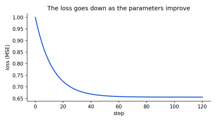
Watch the numbers. The loss drops from 1.0 to 0.656 and then stops improving, because that is the best a straight line through BMI alone can do. And settles near 0.58. That is not a coincidence: with both columns standardised, the best slope of a simple line is exactly the correlation between them, which for BMI and the target is 0.586. The loop found a number you could have calculated in one line, and that is the point. Libraries like scikit-learn solve a straight line directly. This loop matters because it is the same machinery that trains the large models later, where no direct formula exists.
One more thing hiding in that script. I standardised BMI before the loop. Try deleting that line and the same loop crawls, because the raw column is tiny (around 0.05) and the gradients come out tiny too. That is the practical reason scaling matters, and we return to it in Session 5.
In the training loop above, which of these is a parameter?
Parameters, activations and why size matters
A parameter is a number inside the model that training adjusts. In a neural network the parameters are the weights (how strongly one neuron listens to another) and the biases (a shift). They change during training and stay frozen when you use the model to predict.
There is a common mix-up worth clearing. The values flowing through the neurons while a prediction is made are called activations, and they are not parameters. They are recomputed for every input. Parameters are the stored knowledge, activations are the scratch work.
For a fully connected layer, counting parameters is simple multiplication:
One weight for every input-output pair, plus one bias per output. A layer from 10 inputs to 16 neurons has parameters.
import torch.nn as nn
import torchvision

def count(m, trainable_only=False):
    return sum(p.numel() for p in m.parameters() if p.requires_grad or not trainable_only)

# a tiny network: 10 inputs -> 16 hidden -> 1 output
mlp = nn.Sequential(nn.Linear(10, 16), nn.ReLU(), nn.Linear(16, 1))
print("tiny MLP parameters:", count(mlp))          # (10*16 + 16) + (16*1 + 1)

# ResNet-18 (weights=None skips the download; the parameter count is the same)
net = torchvision.models.resnet18(weights=None)
print("resnet18 parameters:", f"{count(net):,}")

# transfer learning: freeze everything, then give it a new 3-class head
for p in net.parameters():
    p.requires_grad = False
net.fc = nn.Linear(net.fc.in_features, 3)
print("trainable after freezing + new head:", count(net, trainable_only=True))tiny MLP parameters: 193
resnet18 parameters: 11,689,512
trainable after freezing + new head: 1539The tiny network has 193 parameters. ResNet-18, a well-known image model, has 11,689,512. More parameters mean more capacity to learn subtle patterns, and also more memory, more electricity and more data needed to avoid memorising. Large language models are in a different league entirely: the GPT-3 paper reported 175 billion parameters.
GPT-3 had about 175 billion parameters. ResNet-18 has about 11.7 million. That is roughly 15,000 times more.GPT-3 paper (Brown et al., 2020); ResNet-18 count computed above
Transfer learning: do not start from zero
Training a big network from scratch needs a mountain of data, a lot of compute and patience. Often you have none of the three. Transfer learning is the shortcut: take a network someone already trained on a huge dataset and reuse what it learned for your smaller problem.
Here is how it works. The early layers of an image network learn general things, like edges and textures, that are useful for almost any picture. So you freeze those layers (stop them changing), cut off the final layer that was built for the old task, attach a fresh one for your own labels, and train only that new part. If you have more data, you can later unfreeze a few of the last frozen layers and fine-tune them gently.
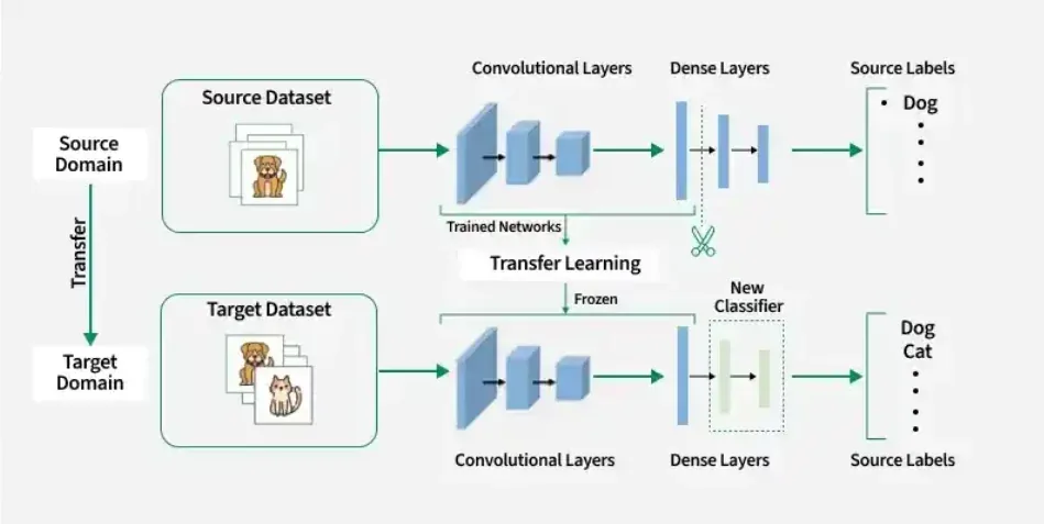
Look back at the output of the parameter count. After freezing and attaching a new 3-class head, only 1,539 of those 11.7 million parameters are trainable: 512 inputs times 3 classes plus 3 biases. That is why transfer learning is fast and works with a few hundred photos.
import torch.nn as nn
import torchvision

model = torchvision.models.resnet18(weights="DEFAULT")   # pre-trained on ImageNet
for p in model.parameters():
    p.requires_grad = False                               # freeze the feature extractor
model.fc = nn.Linear(model.fc.in_features, 3)             # new trainable head: 3 classes
The weights="DEFAULT" line downloads the pre-trained weights the first time you run it, so it needs an internet connection.
The ResNet-18 weights you download were trained on ImageNet-1K, about 1.28 million photos in 1,000 classes. The full ImageNet collection holds over 14 million images, and you borrow all that learning for free.image-net.org / ILSVRC 2012 statistics
Saving your model
Training takes time, so you save the result and reload it later. The format depends on the library, and the choice matters more than it looks.
| Format | Used by | What to know |
|---|---|---|
.pkl (via joblib or pickle) |
scikit-learn | Simple and fast. Pickle can run code when loaded, so never load a .pkl from a source you do not trust. |
.pt / .pth |
PyTorch | Save the state_dict (just the weights) and rebuild the class in code. Smaller and safer than saving the whole object. |
.keras / .h5 |
Keras / TensorFlow | .keras is the current format. .h5 is the older one and still works. |
.safetensors |
Hugging Face | Weights only, no code execution, fast to load. The common choice for shared transformer models. |
.onnx |
Many frameworks | A neutral format, handy for moving a model between tools or to production runtimes. |
.gguf |
llama.cpp | Quantised language models you run on an ordinary CPU. We use it in Session 23. |
import os, tempfile
import joblib
import numpy as np
import torch
from sklearn.datasets import load_diabetes
from sklearn.linear_model import LinearRegression

X, y = load_diabetes(return_X_y=True)
model = LinearRegression().fit(X, y)

d = tempfile.mkdtemp()
joblib.dump(model, f"{d}/model.pkl")                       # scikit-learn model -> .pkl
restored = joblib.load(f"{d}/model.pkl")
print("same predictions after reload:", np.allclose(model.predict(X), restored.predict(X)))
print("model.pkl size:", os.path.getsize(f"{d}/model.pkl"), "bytes")

net = torch.nn.Linear(10, 1)
torch.save(net.state_dict(), f"{d}/net.pt")                # PyTorch: save only the weights
net2 = torch.nn.Linear(10, 1)
net2.load_state_dict(torch.load(f"{d}/net.pt"))
print("net.pt size:", os.path.getsize(f"{d}/net.pt"), "bytes")same predictions after reload: True
model.pkl size: 712 bytes
net.pt size: 1472 bytesThe check at the end is a habit worth keeping: after reloading, confirm the predictions match. A silent mismatch in production is a painful way to find a version problem.
Which model for which data
You do not need to memorise algorithms yet, but you should know the rough map, because choosing well is half of practical machine learning. It is a short version of the table in the course's mind-map chapter.
| Your data | A good place to start |
|---|---|
| A number to predict, roughly linear | Linear regression (Session 2) |
| Rows and columns, a category to predict | Random Forest or XGBoost (Sessions 12 and 13) |
| Images | A CNN (Session 16) |
| Text, code, long sequences | A Transformer (Session 20) |
| Answers from your own documents | RAG on top of an LLM (Session 22) |
Gartner's September 2026 forecast puts worldwide AI spending at about $2.67 trillion this year, up roughly 49.5% from 2025.Gartner press release, 16 September 2026
Try it yourself
Do these in order, and type the code instead of pasting it. It is slower and it works.
- Create the virtual environment and open JupyterLab or Colab.
- Load the diabetes dataset into a DataFrame. Draw a histogram of two other columns besides
bmi. - Make your own messy table with a missing value and a duplicate, and clean it with the steps above.
- Split with
random_state=7instead of 42. Does the R² change? By how much? (It will, and that wobble is itself a lesson about small test sets.) - Save a trained model two ways, for example
.pklandtorch.save, reload both and check the predictions match.
What comes next
You now have the toolkit: an environment, clean data, an honest split and a feel for the training loop. In Session 2 we put a name on the bigger picture, how AI, machine learning, deep learning and generative AI relate to each other, and then build the first real model: linear regression.
Frequently asked questions
Do I need a GPU to learn machine learning?
Not for this Part. Linear models, trees and the small neural networks in Part II run comfortably on a normal laptop CPU. You start to want a GPU around Part IV (images and sequences). Free options like Google Colab cover that when you get there.
What is the difference between a parameter and a hyperparameter?
Parameters are numbers the model learns from the data, like the slope w in a line or the weights in a neural network. Hyperparameters are settings you choose before training, like the learning rate, the number of epochs or how deep a tree is allowed to grow. Session 5 covers tuning them.
Why do I need a separate test set?
Because a model can score perfectly on data it has already seen simply by memorising it. The test set is data it has never touched, so the score on it is an honest estimate of how the model will behave on new data.
What is data leakage in machine learning?
Leakage is when information from outside the training data, usually from the test set, sneaks into training. A classic case is scaling or imputing on the full dataset before splitting. It makes scores look better than they really are, so always split first and fit preprocessing on training rows only, ideally inside a Pipeline.
Is it safe to load a .pkl model file from the internet?
No. Python's pickle format can execute arbitrary code when loaded, so only load pickle files you created or fully trust. For shared models, prefer formats that store only weights, such as safetensors.