Forward and Backpropagation Explained: A Worked Example and a Neural Network from Scratch

Every neural network you will meet in this course, from a handwriting reader to a chat model with hundreds of billions of weights, learns through the same two moves. A forward pass that makes a prediction, and a backward pass that works out how to improve. In Session 9 both happened invisibly inside loss.backward().

Today we open that box. We compute every number of a tiny network by hand, check the result against brute force, and then build a complete network from nothing but NumPy and watch it learn a problem a straight line can never solve. If backpropagation has ever felt like magic, this is the session that turns it into arithmetic.

You need the pieces from the last four sessions: the loss (6), the update rule (7) and the chain-rule idea behind vanishing gradients (8).

Forward propagation

For each layer the network does two things, in this order:

1. Weighted sum: multiply the inputs by the weights and add the bias.
2. Activation: pass the sum through a function such as sigmoid or ReLU.

The output of one layer becomes the input of the next. The last layer gives the prediction $\hat{y}$, and the loss compares it with the true label $y$.

And the loss for this worked example, with a small $\tfrac12$ in front so the derivative comes out clean:

Backpropagation: how much did each weight contribute?

After the forward pass we have an error. Backpropagation answers one question for every single weight: if I nudge this weight slightly, how much does the loss change? That quantity is the weight's gradient, $\partial L/\partial w$.

A network is a chain of functions (sum, activation, sum, activation, loss), so the chain rule of calculus gives the answer by multiplying local slopes while walking backwards from the loss. Each layer reuses the work of the layer after it, which is why it is fast.

Define the "error signal" at a layer as $\boldsymbol{\delta}^{(l)} = \partial L / \partial \mathbf{z}^{(l)}$. Then the whole algorithm is four lines:

Finally the update from Session 7 applies to every weight:

A worked example with real numbers

Theory is easy to nod along to. Let's compute everything for one training example in a tiny network: 2 inputs, 2 hidden neurons (sigmoid), 1 output neuron (sigmoid). The input is $\mathbf{x} = (1.0,\ 0.5)$ and the true label is $y = 1$.

import numpy as np

sigmoid = lambda z: 1 / (1 + np.exp(-z))

# One example, a tiny network: 2 inputs -> 2 hidden (sigmoid) -> 1 output (sigmoid)
x = np.array([1.0, 0.5])
y = 1.0
W1 = np.array([[0.4, -0.6], [0.2, 0.9]])      # row i = weights from input i
b1 = np.array([0.1, -0.2])
W2 = np.array([[0.7], [-0.3]]); b2 = np.array([0.05])

# ---- forward pass ----
z1 = x @ W1 + b1;        a1 = sigmoid(z1)
z2 = a1 @ W2 + b2;       y_hat = sigmoid(z2)
loss = 0.5 * (y - y_hat) ** 2
print("hidden sums   z1 =", z1.round(4))
print("hidden output a1 =", a1.round(4))
print("output sum    z2 =", round(float(z2[0]), 4), "  prediction y_hat =", round(float(y_hat[0]), 4))
print("loss =", round(float(loss[0]), 4))

# ---- backward pass (chain rule, one layer at a time) ----
d_out = (y_hat - y) * y_hat * (1 - y_hat)         # dL/dz2
dW2 = np.outer(a1, d_out); db2 = d_out
d_hid = (W2 @ d_out) * a1 * (1 - a1)              # dL/dz1  (push back through W2, then the sigmoid slope)
dW1 = np.outer(x, d_hid); db1 = d_hid
print("\ndL/dz2 =", d_out.round(4))
print("dL/dW2 =", dW2.ravel().round(4))
print("dL/dW1 =\n", dW1.round(4))

# ---- check the chain rule against brute force: nudge one weight and re-measure ----
def L(W1_):
    return float(0.5 * (y - sigmoid(sigmoid(x @ W1_ + b1) @ W2 + b2)) ** 2)
eps = 1e-6
W1_nudged = W1.copy(); W1_nudged[0, 0] += eps
numeric = (L(W1_nudged) - L(W1)) / eps
print(f"\ndL/dW1[0,0]  backprop: {dW1[0, 0]:.6f}   numerical: {numeric:.6f}")

# ---- one update ----
lr = 0.5
W1_new, b1_new = W1 - lr * dW1, b1 - lr * db1
W2_new, b2_new = W2 - lr * dW2, b2 - lr * db2
y_hat_new = sigmoid(sigmoid(x @ W1_new + b1_new) @ W2_new + b2_new)
print("prediction after one step:", round(float(y_hat_new[0]), 4), "(was 0.5934, target 1.0)")
print("loss after one step      :", round(float(0.5 * (y - y_hat_new[0]) ** 2), 4))

hidden sums   z1 = [ 0.6  -0.35]
hidden output a1 = [0.6457 0.4134]
output sum    z2 = 0.3779   prediction y_hat = 0.5934
loss = 0.0827

dL/dz2 = [-0.0981]
dL/dW2 = [-0.0633 -0.0406]
dL/dW1 =
 [[-0.0157  0.0071]
 [-0.0079  0.0036]]

dL/dW1[0,0]  backprop: -0.015712   numerical: -0.015712
prediction after one step: 0.6129 (was 0.5934, target 1.0)
loss after one step      : 0.0749

Follow it through.

Forward. The hidden sums are 0.6 and -0.35. The sigmoid squeezes them to 0.6457 and 0.4134. The output sum is 0.3779, giving a prediction of 0.5934. The target was 1, so the loss is 0.0827. The network is not very sure.

Backward. Start at the output. The error signal is $(\hat{y}-y)\,\hat{y}(1-\hat{y}) = -0.0981$. The minus sign means "the output should go up". Multiply by the hidden activations to get the output-layer weight gradients (-0.0633 and -0.0406). Now push the error one layer back through the weights and the sigmoid slope, and you get the first-layer weight gradients. Notice how small they are (around -0.016 to 0.007): they are scaled by two sigmoid slopes, the effect from Session 8.

The check. Here is a way to be sure we have not fooled ourselves. Nudge one weight by a tiny amount, re-run the forward pass and see how the loss moved. That brute-force estimate, -0.015712, matches the backpropagation answer, -0.015712, exactly. This habit is called a gradient check, and it is how people catch bugs when they write backprop by hand.

The step. One update with a learning rate of 0.5 moves the prediction from 0.5934 to 0.6129, closer to the target, and the loss drops from 0.0827 to 0.0749. One tiny step. Repeat it thousands of times and the network learns.

Why you need a hidden layer: XOR

XOR ("exclusive or") outputs 1 only when its two inputs differ: (0,0) gives 0, (0,1) gives 1, (1,0) gives 1, (1,1) gives 0. It looks trivial, and it famously cannot be solved by any straight line.

import numpy as np
from sklearn.linear_model import LogisticRegression

X = np.array([[0, 0], [0, 1], [1, 0], [1, 1]])
y = np.array([0, 1, 1, 0])
line = LogisticRegression(C=1e6).fit(X, y)           # a straight-line model, barely regularised
print("straight-line model, accuracy on XOR:", line.score(X, y))
print("its predictions:", line.predict(X))

straight-line model, accuracy on XOR: 0.5
its predictions: [0 0 0 0]

The straight-line model scores 0.5 and predicts 0 for every input, no better than a coin. In 1969, Marvin Minsky and Seymour Papert pointed out that single-layer networks cannot solve XOR, which contributed to a long lull in neural-network research. A hidden layer fixes it, because the hidden neurons can each learn a different straight cut and the output neuron combines them into a curved decision. But the hidden layer needs a way to learn, and backpropagation is exactly what makes that possible.

A network from scratch in NumPy

Here is the complete thing: forward pass, backward pass and update, with no deep-learning library at all. It uses 4 hidden sigmoid neurons and trains for 5,000 epochs.

import numpy as np
import matplotlib.pyplot as plt

rng = np.random.default_rng(0)
X = np.array([[0, 0], [0, 1], [1, 0], [1, 1]], dtype=float)
y = np.array([[0], [1], [1], [0]], dtype=float)      # XOR: 1 only when the inputs differ

W1 = rng.normal(0, 1, (2, 4)); b1 = np.zeros((1, 4))   # input -> hidden
W2 = rng.normal(0, 1, (4, 1)); b2 = np.zeros((1, 1))   # hidden -> output
sigmoid = lambda z: 1 / (1 + np.exp(-z))
lr = 0.5
losses = []

for epoch in range(5000):
    # forward pass
    h = sigmoid(X @ W1 + b1)
    y_hat = sigmoid(h @ W2 + b2)
    loss = np.mean((y - y_hat) ** 2)
    losses.append(loss)

    # backward pass (chain rule)
    d_out = 2 * (y_hat - y) / len(X) * y_hat * (1 - y_hat)
    dW2 = h.T @ d_out;   db2 = d_out.sum(0, keepdims=True)
    d_hid = d_out @ W2.T * h * (1 - h)
    dW1 = X.T @ d_hid;   db1 = d_hid.sum(0, keepdims=True)

    # update
    W1 -= lr * dW1; b1 -= lr * db1
    W2 -= lr * dW2; b2 -= lr * db2
    if epoch in (0, 500, 1000, 2000, 4999):
        print(f"epoch {epoch:4d}   loss {loss:.4f}")

print("\ninputs -> prediction")
for xi, p in zip(X, sigmoid(sigmoid(X @ W1 + b1) @ W2 + b2)):
    print(f"  {xi.astype(int)} -> {p[0]:.3f}")

fig, ax = plt.subplots(figsize=(6, 3.4))
ax.plot(losses, color="#7C3AED", lw=2); ax.set_xlabel("epoch"); ax.set_ylabel("loss (MSE)")
ax.spines[["top", "right"]].set_visible(False)
fig.tight_layout()

epoch    0   loss 0.3430
epoch  500   loss 0.2475
epoch 1000   loss 0.2188
epoch 2000   loss 0.0233
epoch 4999   loss 0.0022

inputs -> prediction
  [0 0] -> 0.020
  [0 1] -> 0.952
  [1 0] -> 0.952
  [1 1] -> 0.061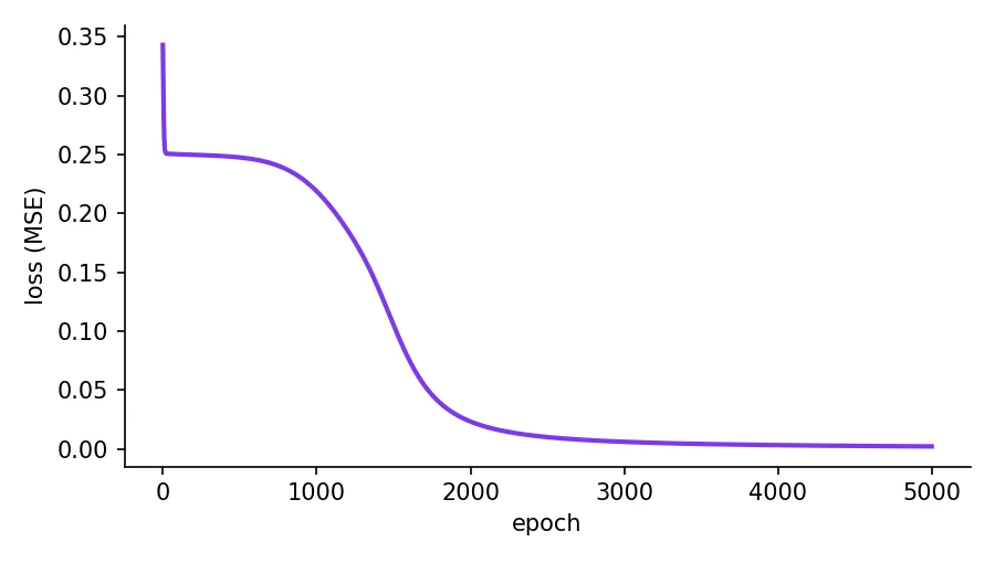

Read the print-out like a diary. For the first thousand epochs the loss barely moves (0.343, 0.2475, 0.2188): the network is stuck on a plateau, guessing 0.5 for everything. Between epochs 1000 and 2000 it finds the pattern and the loss collapses to 0.0233, and by epoch 5000 it is 0.0022. The predictions confirm it: (0,0) gives 0.020, (0,1) gives 0.952, (1,0) gives 0.952, (1,1) gives 0.061. That is XOR, learned from nothing but a random start.

Notice that every line of the backward pass is one of the four equations above:

• d_out is the output-layer error signal (equation 1).
• d_hid = d_out @ W2.T * h * (1 - h) pushes the error back through the weights and the sigmoid slope (equation 2).
• dW2, dW1 are the weight gradients (equation 3), and db2, db1 the bias gradients (equation 4).

The same thing in PyTorch: autograd

Writing the chain rule by hand is a great way to learn it and a terrible way to build a 50-layer network. Libraries do it for you with automatic differentiation ("autograd"). While the forward pass runs, PyTorch quietly records every operation, and loss.backward() replays that record backwards applying the chain rule.

import torch
import torch.nn as nn

torch.manual_seed(0)
X = torch.tensor([[0., 0.], [0., 1.], [1., 0.], [1., 1.]])
y = torch.tensor([[0.], [1.], [1.], [0.]])
net = nn.Sequential(nn.Linear(2, 4), nn.Sigmoid(), nn.Linear(4, 1), nn.Sigmoid())
opt = torch.optim.SGD(net.parameters(), lr=0.5)
loss_fn = nn.MSELoss()

for epoch in range(5000):
    loss = loss_fn(net(X), y)    # forward pass + loss
    opt.zero_grad()
    loss.backward()              # backpropagation: PyTorch does the chain rule for us
    opt.step()                   # parameter update

print("final loss:", round(loss.item(), 4))
print("predictions:", net(X).detach().numpy().round(2).ravel())

final loss: 0.0019
predictions: [0.04 0.96 0.96 0.04]

It reaches the same place, a loss of 0.0019 and predictions of 0.04 and 0.96, with the whole backward pass replaced by one call. The two lines opt.zero_grad() and opt.step() are the gradient reset and the update rule from Session 7. This is the pattern you will see in every training loop for the rest of the course.

Why this matters for everything that follows

The rest of the course changes the shape of the network, not this loop. A convolutional network (Session 16) shares weights across an image. A recurrent network (Session 18) loops its hidden state through time. A Transformer (Session 20) replaces both with attention. A large language model (Session 21) is that Transformer at enormous scale. Every one of them is trained by the same cycle:

forward pass, loss, backpropagation, parameter update.

If you can explain that cycle, and you now can, you understand the engine behind modern AI.

Try it yourself

1. In worked_example.py, change the true label to $y = 0$. Which way do the gradients point now?
2. Run xor_numpy.py with 2 hidden neurons, then 8. Does it still learn XOR? How does the number of epochs it needs change?
3. Change the activation from sigmoid to ReLU in the PyTorch version. Does it still solve XOR with 4 hidden neurons?
4. Write a gradient check for one weight in xor_numpy.py: nudge it by 1e-5, measure the loss change and compare with the analytic gradient.

Part II complete: what you can do now

You can define what "wrong" means (loss), bend a network's output (activations), walk downhill efficiently (gradient descent and its optimisers), spot and fix vanishing gradients, and explain exactly how a network computes its predictions and its gradients. That is the entire training story of a neural network.

Part III takes the other road to non-linearity. Instead of stacking neurons, we split data with simple questions. Session 11 starts with the decision tree, the most readable model in machine learning.

Frequently asked questions