
A random forest asks hundreds of trees to work in parallel and then votes. Boosting does something different and, on tables of numbers, often better: it builds the trees one after another, and each new tree is trained specifically to fix the mistakes of the ones before it. Think of a student who takes a practice test, studies only the questions they got wrong, takes another test and repeats.
If you ever enter a data-science competition or work with business tables, this session covers the family you will use most: AdaBoost, gradient boosting, XGBoost and LightGBM. We build gradient boosting from scratch in a few lines so that nothing is a black box. At the end there is a short bonus on reinforcement learning and RLHF, a vocabulary you will need again in Session 21. This session builds on the trees of Session 11 and the forest of Session 12.
Bagging versus boosting
Both are ensembles: a team of models that beats any single member. They attack different errors.
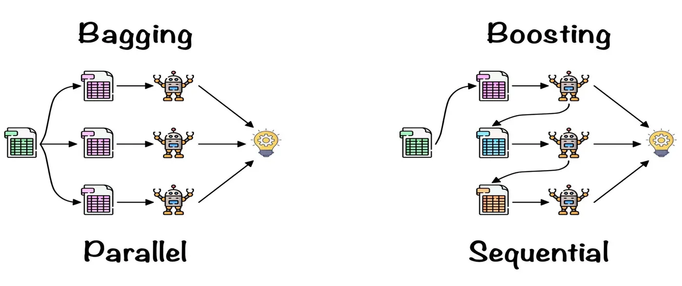
Recall the two ways a model fails from Session 3: bias (too simple, systematically misses the pattern, underfits) and variance (too sensitive to the training sample, overfits). Bagging, as in a forest, reduces variance. Boosting reduces bias, by chaining many deliberately simple models, usually small trees, into one expressive one.
| Bagging | Boosting | |
|---|---|---|
| Training | Independent models, in parallel | Sequential, each waits for the last |
| Main goal | Reduce variance | Reduce bias |
| Treatment of rows | All rows equal | Hard rows get more attention |
| Overfitting | Hard to overfit | More prone to it without care |
| Noise and outliers | Less affected | Sensitive |
| Example | Random forest | XGBoost |
Boosting from scratch
Here is the core idea of gradient boosting for a regression problem, in four steps:
- Start with a trivial model: always predict the average of the target.
- Compute the residuals: the gap between each real value and the current prediction.
- Train a small tree to predict those residuals.
- Add a fraction of that tree's output to the prediction. Go back to step 2.
is the model after trees, the new small tree fitted to the residuals and ("eta") the learning rate, usually 0.01 to 0.3. A small means each tree makes only a modest correction, which makes the result smoother and less prone to overfitting.
Why is it called gradient boosting? For squared error, the residual is exactly the negative gradient of the loss with respect to the prediction. Fitting residuals is gradient descent, but in the space of functions, with each tree as a step. That is the link to Session 7: it is the same idea, applied to models instead of weights.
For any other differentiable loss, the new tree is fitted to that loss's negative gradient instead. That is what makes the method general, and why the same recipe works for classification and ranking.
import numpy as np
import matplotlib.pyplot as plt
from sklearn.tree import DecisionTreeRegressor

rng = np.random.default_rng(0)
x = np.sort(rng.uniform(0, 6, 120)); y = np.sin(x) + rng.normal(0, 0.2, 120)
X = x.reshape(-1, 1)

lr = 0.3
pred = np.full_like(y, y.mean())          # start from the laziest model: always the average
trees = []
grid = np.linspace(0, 6, 300).reshape(-1, 1)
snapshots = {}
for round_ in range(1, 61):
    residual = y - pred                                    # what we still get wrong
    stump = DecisionTreeRegressor(max_depth=2).fit(X, residual)   # a small tree that predicts the mistakes
    pred = pred + lr * stump.predict(X)                    # add a fraction of its correction
    trees.append(stump)
    if round_ in (1, 5, 20, 60):
        mse = np.mean((y - pred) ** 2)
        print(f"after {round_:2d} trees   training MSE {mse:.4f}")
        snapshots[round_] = y.mean() + lr * sum(t.predict(grid) for t in trees)

fig, ax = plt.subplots(1, 4, figsize=(12, 3), sharey=True)
for a, (k, g) in zip(ax, snapshots.items()):
    a.scatter(x, y, s=8, color="#9CA3AF"); a.plot(grid, g, color="#DC2626", lw=2); a.set_title(f"{k} tree{'s' if k > 1 else ''}")
    a.spines[["top", "right"]].set_visible(False)
fig.tight_layout()after 1 trees training MSE 0.2899
after 5 trees training MSE 0.0634
after 20 trees training MSE 0.0245
after 60 trees training MSE 0.0093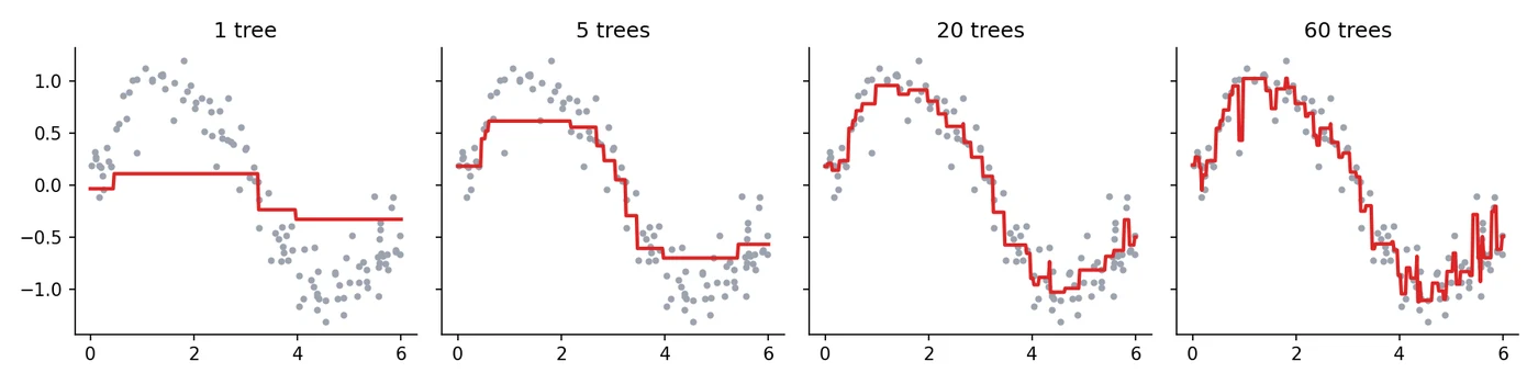
Watch the training error: 0.2899 after one tree, 0.0634 after five, 0.0245 after twenty and 0.0093 after sixty. In the figure, one tree gives a crude staircase and sixty trees trace the sine curve, though the last panel already shows jagged spikes where the model starts chasing noise. Each tree is tiny (depth 2) and individually weak. The strength is in the sum.
Gradient boosting was formalised by Jerome Friedman in 2001. Its ancestor AdaBoost, by Yoav Freund and Robert Schapire, won the Gödel Prize in 2003 for its theoretical impact.Friedman, 2001; Freund and Schapire, 1997
AdaBoost: re-weighting the rows
AdaBoost (adaptive boosting) was the first successful boosting algorithm. Instead of fitting residuals, it re-weights the training rows: rows the current model gets wrong are given more weight, so the next learner is forced to pay attention to them. The learners are often stumps, trees with a single question.
is the weighted error of learner , so a more accurate learner gets a bigger vote . Labels are . When a learner is right () the row's weight shrinks, and when it is wrong the weight grows. The final prediction is a weighted vote of all learners.
from sklearn.datasets import load_breast_cancer
from sklearn.ensemble import AdaBoostClassifier
from sklearn.model_selection import cross_val_score
from sklearn.tree import DecisionTreeClassifier

X, y = load_breast_cancer(return_X_y=True)
stump = DecisionTreeClassifier(max_depth=1)                     # one single yes/no question
print("one stump                :", round(cross_val_score(stump, X, y, cv=5).mean(), 3))
for n in (10, 50, 200):
    ada = AdaBoostClassifier(estimator=DecisionTreeClassifier(max_depth=1), n_estimators=n, random_state=0)
print(f"AdaBoost of {n:3d} stumps :", round(cross_val_score(ada, X, y, cv=5).mean(), 3))one stump : 0.903
AdaBoost of 10 stumps : 0.94
AdaBoost of 50 stumps : 0.972
AdaBoost of 200 stumps : 0.975A single stump, one yes/no question, scores 90.3 percent. Ten stumps boosted together reach 94.0, fifty reach 97.2 and two hundred 97.5. Individually the stumps are barely better than a coin on the hard cases. Combined, with each concentrating on what the last missed, they become a serious model.
XGBoost, LightGBM and CatBoost
Plain gradient boosting is slow and easy to overfit. A family of engineering improvements turned it into the default for tabular data.
- XGBoost (eXtreme Gradient Boosting) is a fast, regularised implementation. It adds L1 and L2 penalties on the leaf values, row and column subsampling, tree pruning and parallel computation.
- LightGBM, from Microsoft, grows trees leaf-wise (always splitting the leaf that helps most) with a histogram-based method, which makes it very fast and light on memory for large data.
- CatBoost, from Yandex, handles categorical columns automatically and uses ordered boosting to avoid target leakage.
XGBoost's objective makes the regularisation explicit:
The first sum is the usual loss over all rows. The second penalises each tree : is its number of leaves, the value in leaf , a cost per leaf and the L2 strength. It is the same "pay for complexity" idea as Ridge in Session 3, built into every tree.
In the XGBoost paper, the authors reported that among the 29 winning solutions published on Kaggle's blog in 2015, 17 used XGBoost, and eight of those used it on its own.Chen and Guestrin, XGBoost: A Scalable Tree Boosting System, KDD 2016
How do they compare?
Same breast-cancer data and the same repeated cross-validation as last session.
import numpy as np
from lightgbm import LGBMClassifier
from sklearn.datasets import load_breast_cancer
from sklearn.ensemble import GradientBoostingClassifier, RandomForestClassifier
from sklearn.model_selection import RepeatedStratifiedKFold, cross_val_score
from xgboost import XGBClassifier

X, y = load_breast_cancer(return_X_y=True)
cv = RepeatedStratifiedKFold(n_splits=5, n_repeats=3, random_state=0)
models = {
    "random forest":            RandomForestClassifier(n_estimators=300, random_state=0, n_jobs=-1),
    "gradient boosting (sklearn)": GradientBoostingClassifier(n_estimators=200, learning_rate=0.1, max_depth=3, random_state=0),
    "XGBoost":                  XGBClassifier(n_estimators=300, learning_rate=0.05, max_depth=3, subsample=0.8, colsample_bytree=0.8, eval_metric="logloss", random_state=0),
    "LightGBM":                 LGBMClassifier(n_estimators=300, learning_rate=0.05, num_leaves=15, random_state=0, verbose=-1),
}
for name, m in models.items():
    s = cross_val_score(m, X, y, cv=cv)
print(f"{name:30s} accuracy {s.mean():.3f} (+/- {s.std():.3f})")random forest accuracy 0.960 (+/- 0.012)
gradient boosting (sklearn) accuracy 0.963 (+/- 0.013)
XGBoost accuracy 0.967 (+/- 0.014)
LightGBM accuracy 0.964 (+/- 0.012)All four land between 96.0 and 96.7 percent, and the error bars (about 1.2 to 1.4 points) overlap completely. On a small, easy dataset like this, no method is meaningfully better, and honest comparison means saying so. The advantage of boosting shows on larger, messier tables, where a tuned XGBoost or LightGBM very often tops the leaderboard.
Controlling a booster
Boosting is flexible enough to overfit, and its main dial is the interplay of two settings: learning rate and number of trees. A small learning rate with many trees is smoother but slower, and the more trees you add, the more you can overfit.
from sklearn.datasets import load_diabetes
from sklearn.ensemble import GradientBoostingRegressor
from sklearn.metrics import r2_score
from sklearn.model_selection import train_test_split

X, y = load_diabetes(return_X_y=True)
X_tr, X_te, y_tr, y_te = train_test_split(X, y, test_size=0.2, random_state=42)

print("learning_rate  n_trees   test R²")
for lr, n in [(1.0, 100), (0.1, 100), (0.1, 500), (0.02, 500), (0.02, 2000)]:
    gb = GradientBoostingRegressor(learning_rate=lr, n_estimators=n, max_depth=2, subsample=0.8, random_state=0).fit(X_tr, y_tr)
print(f" {lr:<8} {n:5d} {r2_score(y_te, gb.predict(X_te)):.3f}")learning_rate n_trees test R²
1.0 100 -0.284
0.1 100 0.424
0.1 500 0.303
0.02 500 0.460
0.02 2000 0.375Read the rows. A learning rate of 1.0 (no shrinking) overfits badly: a test R² of -0.284. At 0.1 with 100 trees it reaches 0.424, but with 500 trees at the same rate it falls to 0.303, because the extra trees chase noise. A gentler 0.02 with 500 trees reaches 0.460, the best here, and 2,000 trees at 0.02 drops again to 0.375. More trees are not always better, which is why you should not guess the number. Let the validation score decide with early stopping.
import matplotlib.pyplot as plt
from sklearn.datasets import load_breast_cancer
from sklearn.model_selection import train_test_split
from xgboost import XGBClassifier

X, y = load_breast_cancer(return_X_y=True)
X_tr, X_rest, y_tr, y_rest = train_test_split(X, y, test_size=0.4, random_state=3, stratify=y)
X_va, X_te, y_va, y_te = train_test_split(X_rest, y_rest, test_size=0.5, random_state=3, stratify=y_rest)   # validation and test kept apart

xgb = XGBClassifier(n_estimators=500, learning_rate=0.1, max_depth=3, subsample=0.8, colsample_bytree=0.8,
                    eval_metric="logloss", early_stopping_rounds=20, random_state=0)
xgb.fit(X_tr, y_tr, eval_set=[(X_tr, y_tr), (X_va, y_va)], verbose=False)

print("asked for 500 trees, stopped after:", len(xgb.evals_result()["validation_0"]["logloss"]))
print("best round:", xgb.best_iteration, "  best validation logloss:", round(xgb.best_score, 4))
print("accuracy on the untouched test set:", round(xgb.score(X_te, y_te), 3))

res = xgb.evals_result()
fig, ax = plt.subplots(figsize=(6.4, 3.7))
ax.plot(res["validation_0"]["logloss"], lw=2, color="#2563EB", label="training")
ax.plot(res["validation_1"]["logloss"], lw=2, color="#F59E0B", label="validation")
ax.axvline(xgb.best_iteration, color="#16A34A", ls="--", label="best round")
ax.set_xlabel("boosting round (trees added)"); ax.set_ylabel("log loss"); ax.legend(frameon=False); ax.spines[["top", "right"]].set_visible(False)
fig.tight_layout()asked for 500 trees, stopped after: 116
best round: 95 best validation logloss: 0.2028
accuracy on the untouched test set: 0.982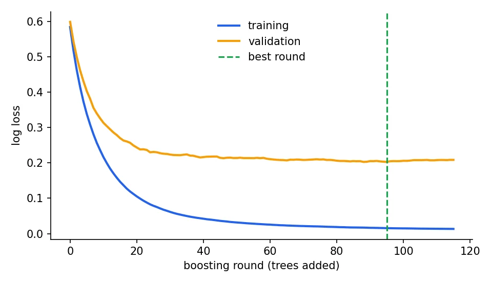
We asked for up to 500 trees. Training stopped after 116 because the validation loss had not improved for 20 rounds, and the model kept the best round (95). Note the careful split here: training data to fit, a separate validation set to decide when to stop, and an untouched test set for the final score (98.2 percent, on only 114 rows, so treat it as noisy). Early-stopping on the test set would quietly leak it, the Session 5 trap.
from sklearn.ensemble import AdaBoostClassifier, GradientBoostingClassifier
from xgboost import XGBClassifier
from lightgbm import LGBMClassifier

ada = AdaBoostClassifier(n_estimators=100, learning_rate=0.5)
gbm = GradientBoostingClassifier(n_estimators=200, learning_rate=0.1, max_depth=3)
xgb = XGBClassifier(n_estimators=300, learning_rate=0.05, max_depth=4,
                    subsample=0.8, colsample_bytree=0.8, reg_lambda=1.0, eval_metric="logloss")
xgb.fit(X_train, y_train, eval_set=[(X_val, y_val)], verbose=False)
lgbm = LGBMClassifier(n_estimators=300, learning_rate=0.05, num_leaves=31)
subsample and colsample_bytree randomly sample rows and columns for each tree (borrowing the forest's trick) and reg_lambda is the L2 penalty from the objective above.
What is the main difference between bagging and boosting?
You lower a booster's learning rate from 0.3 to 0.03. What should you usually do next?
Bonus: a primer on reinforcement learning and RLHF
You have now seen supervised learning (Parts I to III) and unsupervised learning (clustering). There is a third paradigm, reinforcement learning (RL), and a short introduction here pays off later. It returns in Session 21 (how chat models are aligned) and in Sessions 28 to 30 (agents).
In RL there are no labelled answers. An agent takes actions in an environment and receives a reward, a single number saying how good that was. The goal is to learn a strategy that maximises the total reward over time, by trial and error.
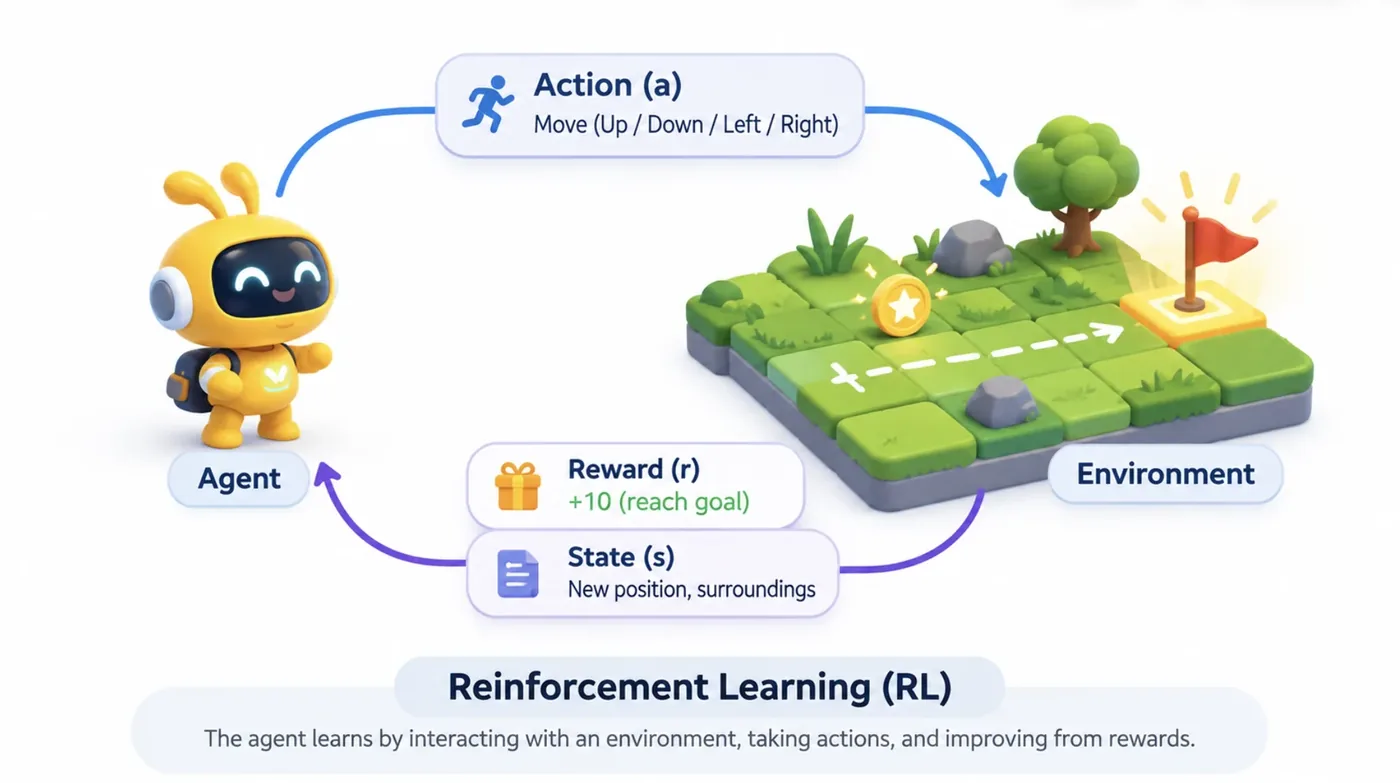
- Agent: the learner and decision-maker (a game-playing program, a chatbot, a robot arm).
- Environment: everything it interacts with.
- State : the current situation the agent can see.
- Action : a choice it makes, such as a move or the next word.
- Reward : the feedback signal.
- Policy : the agent's strategy, a mapping from state to action.
- Value function : an estimate of how much total reward it can expect from a state.
("gamma", between 0 and 1) is the discount factor: a reward now is worth more than the same reward later. The agent's aim is to choose actions that maximise the expected return .
RLHF: teaching a language model what "helpful" means
A freshly pre-trained language model has only learned to predict the next word from internet text. It does not inherently know how to follow instructions, stay honest or avoid harmful output, and writing a mathematical reward for "be helpful, honest and harmless" is nearly impossible. Reinforcement learning from human feedback (RLHF) gets around that by using human judgement as the reward:
- Collect demonstrations. People write good answers to prompts, and the model is fine-tuned on them (supervised fine-tuning).
- Train a reward model. The model produces several answers to a prompt, people rank them, and a separate reward model learns to predict which answer people prefer.
- Optimise with RL. The language model is then tuned with reinforcement learning (typically an algorithm called PPO) to produce answers the reward model scores highly, while a penalty keeps it from drifting too far from the original model.
For a prompt , is the answer people preferred and the one they ranked lower, and is the reward model's score. The loss is small when the preferred answer scores clearly higher. is the sigmoid from Session 6.
OpenAI's 2022 InstructGPT paper showed that a 1.3-billion-parameter model tuned with RLHF was preferred by human raters over the raw 175-billion-parameter GPT-3, a model more than 100 times larger.Ouyang et al., Training language models to follow instructions with human feedback, 2022
Try it yourself
- In
boosting_scratch.py, changemax_depth=2to 1 and then 5. Which gives the best curve after 60 trees, and which overfits? - In
adaboost_stumps.py, run AdaBoost withmax_depth=3base trees instead of stumps. Is it better or worse? - Add
reg_lambda=10to the XGBoost model inxgb_early_stop.py. How do the best round and validation loss change? - Run
learning_rate_vs_trees.pywithsubsample=1.0. Does subsampling help or hurt?
What comes next
We have now covered the two ensemble ideas of tree models: averaging independent trees and chaining dependent ones. Session 14 takes a completely different route to non-linearity: instead of splitting or averaging, it looks for the boundary with the widest possible margin, and uses a clever trick to bend it.
Frequently asked questions
What is boosting in machine learning?
Boosting builds a strong model by training many weak models one after another, where each new model concentrates on the errors of the previous ones. The models are then combined into one prediction. It mainly reduces bias and is the idea behind AdaBoost, gradient boosting, XGBoost and LightGBM.
What is the difference between gradient boosting and XGBoost?
Gradient boosting is the general method of fitting each new tree to the negative gradient of the loss. XGBoost is an optimised implementation of it with built-in regularisation, row and column subsampling, parallel computation and handling of missing values, which makes it faster and usually more accurate.
Should I use XGBoost or LightGBM?
Both are excellent and often give similar accuracy. LightGBM tends to be faster and lighter on very large datasets, while XGBoost is a very solid all-rounder. Try both with cross-validation on your own data, and consider CatBoost if you have many categorical columns.
How do I prevent a boosted model from overfitting?
Use a small learning rate, limit tree depth, subsample rows and columns, add L1 or L2 regularisation, and use early stopping with a separate validation set so the number of trees is chosen automatically.
What is RLHF and why is it used?
Reinforcement learning from human feedback fine-tunes a language model using human preferences. People rank answers, a reward model learns those rankings, and the language model is then optimised with reinforcement learning to produce answers that score highly. It is used because qualities like helpfulness and safety are hard to write as a formula.